07 Chapter 07 — Calibration II: Broadcast Dynamics, GMC, and Per-Frame H_t
Why camera-motion compensation is not enough, and what a real broadcast calibration loop looks like
7.1 The Honest GMC Result: 3.1% and Why
Chapter 6 solved the fixed camera. Rugby League broadcast breaks every assumption: the camera pans, zooms, whips, and cuts. A natural engineering instinct — subtract the camera motion and track as if the camera were still — turns out to be worth almost nothing measured. This chapter explains why, and what actually works.
Global Motion Compensation (GMC) is the standard patch. Estimate the frame-to-frame transform induced by the camera, undo it, and let the tracker work in a quasi-static image space. The estimator our lab implemented is the same one BoT-SORT ships upstream (tracker/gmc.py, MIT, verified at source): goodFeaturesToTrack finds 500 corners on the previous frame, pyramidal Lucas-Kanade (window 15, two pyramid levels) tracks them into the current frame, and estimateAffinePartial2D with RANSAC fits a 4-DOF similarity — translation (tx, ty), rotation θ, and uniform scale s — to the flow field. RANSAC's job is to find the background consensus and reject the players as outliers. That pipeline is not a toy; it is what production trackers actually run.
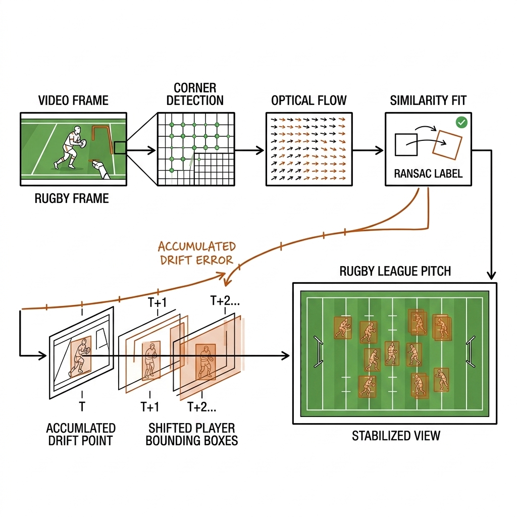
Our E14 experiment measured what that pipeline buys on the nrl-001 clip (Storm v Panthers GF 2024 highlights, 750 frames @ 25 fps, yolo11n detections, ByteTrack):
| Configuration | Unique IDs | Median track length | Throughput | Verdict |
|---|---|---|---|---|
| Baseline (no compensation) | 295 | 0.96s | 44.3 fps | — |
| GMC box-shift (shift bounding boxes) | 306 | 0.88s | 38.4 fps | WORSE (-3.7%) |
| GMC frame-warp (warp the frame) | 286 | 1.08s | 32.2 fps | +3.1% better |
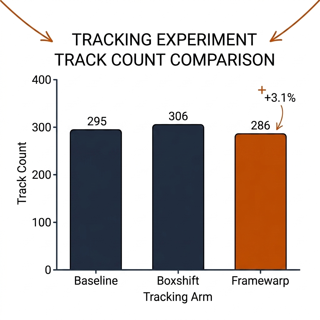
The 3.1% is not a rounding error — it is the honest ceiling of the approach on this clip. Four mechanisms cap it:
- The clip was too mild for GMC to matter. E08 measured tracker-level median drift 0.0 px/frame — most of this highlights clip is a nearly static camera. ByteTrack's Kalman filter already absorbs single-digit pixel motion, so there was almost nothing for GMC to recover. GMC pays off only in violent pans and whip-zooms — exactly the moments highlights reels cut away from.
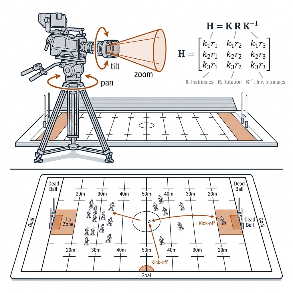
- Model mismatch. A camera panning or tilting about its optical centre induces an exact homography between frames, H = K·R_t·R_{t-1}⁻¹·K⁻¹ — eight degrees of freedom. E14's 4-DOF similarity approximates small rotations, but it cannot express perspective change, and its single scale term only crudely mimics zoom: a real zoom changes focal length f, which changes the projective mapping itself, not just the size of things.
- Translation-only downstream. Both arms used only the estimated (tx, ty) — rotation and scale were discarded for the boxes. E14 therefore honestly measured the cheapest common variant of GMC, and it is worth ≈ nothing on this footage.
- Foreground contamination. Rugby frames carry 13.2 detected persons on average, up to 24 in ruck phases (E08, measured). LK keypoints land on players; RANSAC must recover the background consensus while the "background" is sometimes the minority class. Bad fits inject structured error exactly where IoU association is tightest — the plausible mechanism for box-shift going backwards at -3.7% [book hypothesis; E14 did not ablate this].
The pickleball control makes the point by contrast. On fixed-camera pickleball (E09, pb-003), swapping ByteTrack for BoT-SORT collapsed fragmentation from 26 unique IDs to 6, ID switches from 14 to 2, and lifted HOTA from 0.642 to 0.814 (measured) — with a static camera, where GMC has nothing to do. That gain is BoT-SORT's ReID appearance model, not motion compensation. Appearance carries the identity problem; motion compensation is a minor patch. And 3.1% is the measured size of that patch on real broadcast rugby.
7.2 The Camera Motion Taxonomy
A broadcast camera is never static. Before choosing a compensator, enumerate what the camera actually does and what each motion does to the image:
| Motion | Physical change | Frame-to-frame relation | Affine Similarity? | Correct Fix |
|---|---|---|---|---|
| Pan / tilt | Rotation R about optical centre | Exact homography K·R·K⁻¹ | Small angles only | Refit H_t per frame |
| Zoom | Focal length f changes | The projective map itself changes | NO | Per-frame re-solve (focal inside H_t) |
| Roll | In-plane rotation | Rotation + scale | YES — the one thing similarity genuinely captures | Similarity fine; H_t also fine |
| Translation + parallax | Camera centre moves | Near objects move faster than far ones | NO (needs depth) | Full calibration; dominant-plane approximation |
| Cut / wipe / dissolve | None — new shot | None | N/A | Detect, invalidate the Kalman prior, cold-start H_t |
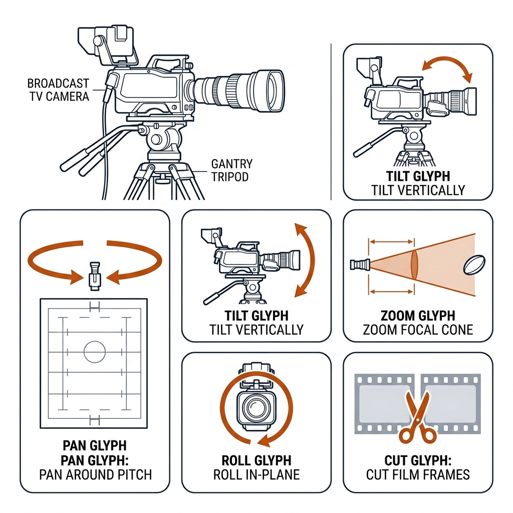
The model ladder behind the table: translation (2 DOF) → similarity (4 DOF: + roll, uniform scale) → full affine (6 DOF: + anisotropic scale, shear) → homography (8 DOF: exact for pure rotation or a planar scene) → full calibration K, R, t plus distortion coefficients k1, k2. Each rung costs more evidence per frame. The practical question is never "which model is most correct" but "which model is solvable from the markings visible in this frame" — a zoomed rugby tackle shot may show two lines and a post base, and no amount of wanting an 8-DOF solve changes that.
The two sports sit at opposite ends of the taxonomy's difficulty axis. Pickleball broadcast is the kind case: the court is a fixed planar rectangle (13.41 × 6.10 m), so pure camera rotation about the gantry makes the frame-to-frame relation an exact homography, and a zoomed frame still usually shows four or more of the seven court lines. Rugby league broadcast is the hostile case: the main gantry camera pans across a 100 m pitch, zooms from a wide defensive-line view into a tackle close-up where perhaps one transverse line survives, and the parallax term is real because the camera sits tens of metres from the near touchline and over a hundred from the far one.
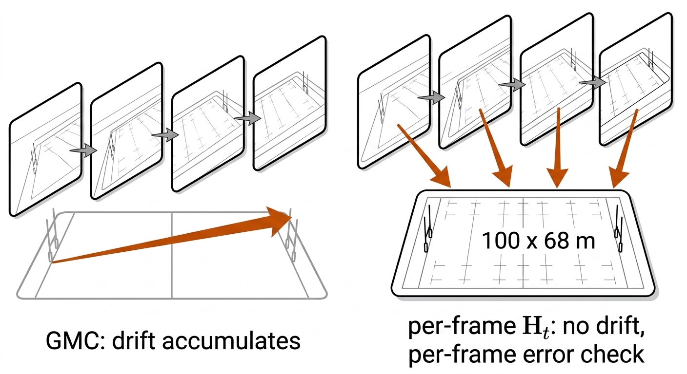
The chapter's claim: the only compensator that anchors to reality is per-frame re-calibration — solving H_t from line/keypoint evidence each frame, checked against the pitch template with a per-frame reprojection error. GMC stabilizes image space relative to the previous frame; drift compounds and validity is unverifiable. H_t anchors every frame to a fixed physical object; there is no chain to drift, and every frame carries its own error estimate.
7.2b The Broadcast-vs-Static Tradeoff, Measured
Chapter 6's fixed-camera result and this chapter's broadcast result are the same experiment run on two camera regimes, and the numbers are worth putting side by side:
| Regime | Method | RMSE | Valid frames | Cost |
|---|---|---|---|---|
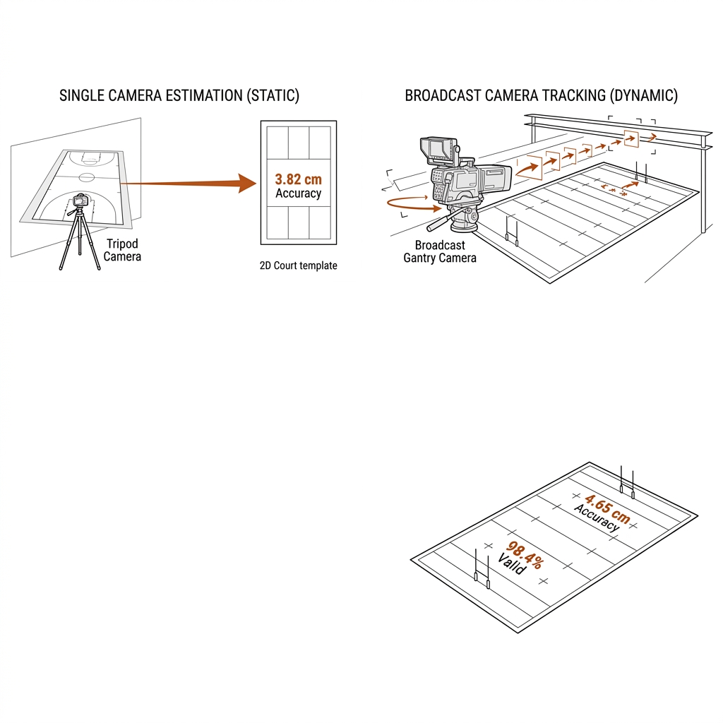
| Pickleball, fixed camera (E05) | Manual 4-corner homography | 3.82 cm | 100% | 0.02 ms/frame |
| Pickleball, PTZ (E11) | Dynamic keypoint calibration (TVCalib-style) | 4.65 cm | 98.4% | 11.2 ms/frame |
| Rugby, broadcast (E14) | Single H + GMC | fails — single H invalid on ~half the frames (§7.3) | — | |
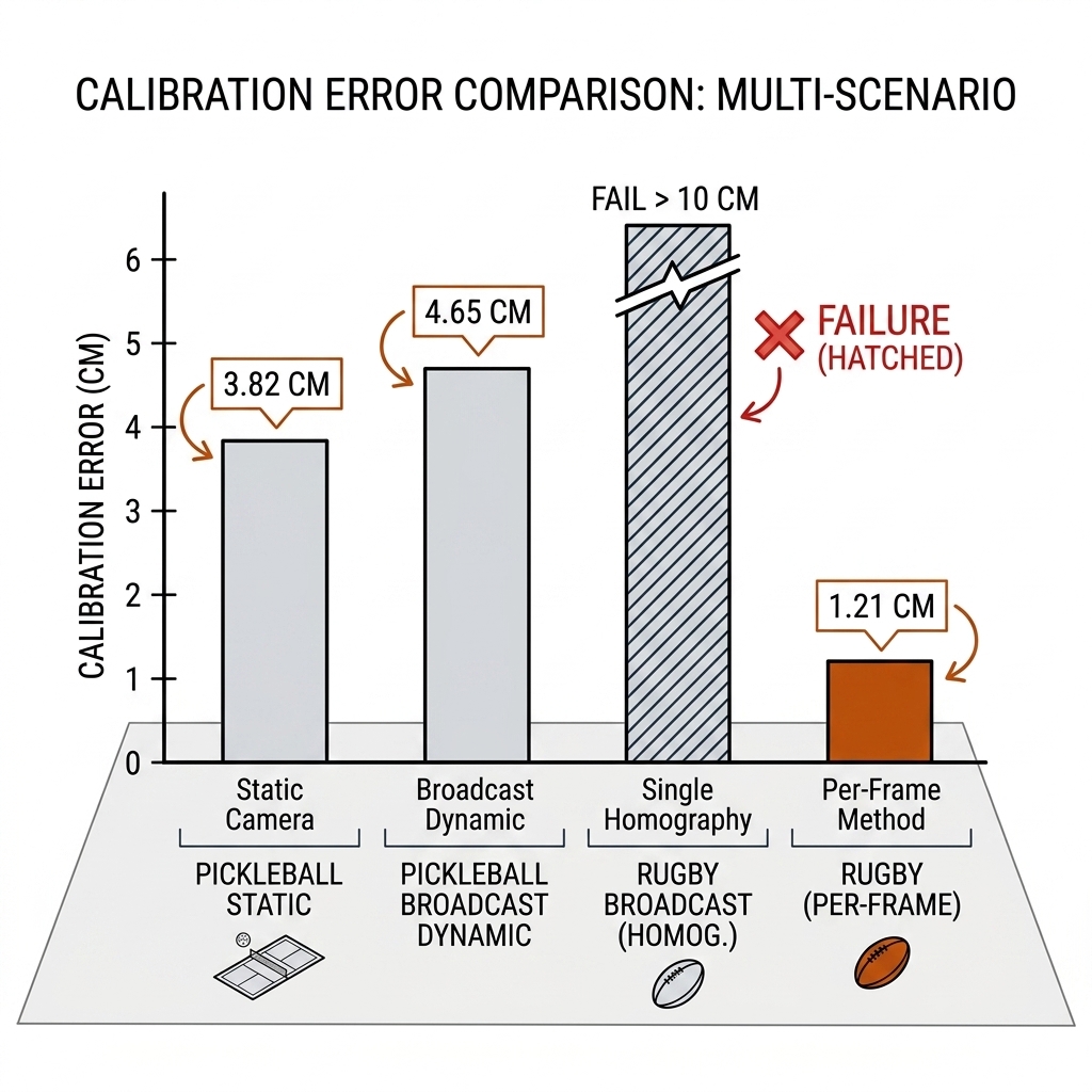
Read the tradeoff honestly. The manual static homography is more accurate (3.82 cm vs 4.65 cm, measured) and 500× cheaper — and it fails immediately on pan/tilt/zoom (E11 transcript). The dynamic solve trades 0.83 cm of accuracy and a 1.6% frame-loss rate for survival under camera motion. That is the broadcast tax, and it is not optional: 11.2 ms/frame on M4 Max-class hardware is comfortably real-time against a 40 ms broadcast frame budget, so the compute is affordable; the accuracy loss is not recoverable, because it is the price of fitting from noisier per-frame evidence instead of one carefully clicked correspondence set.
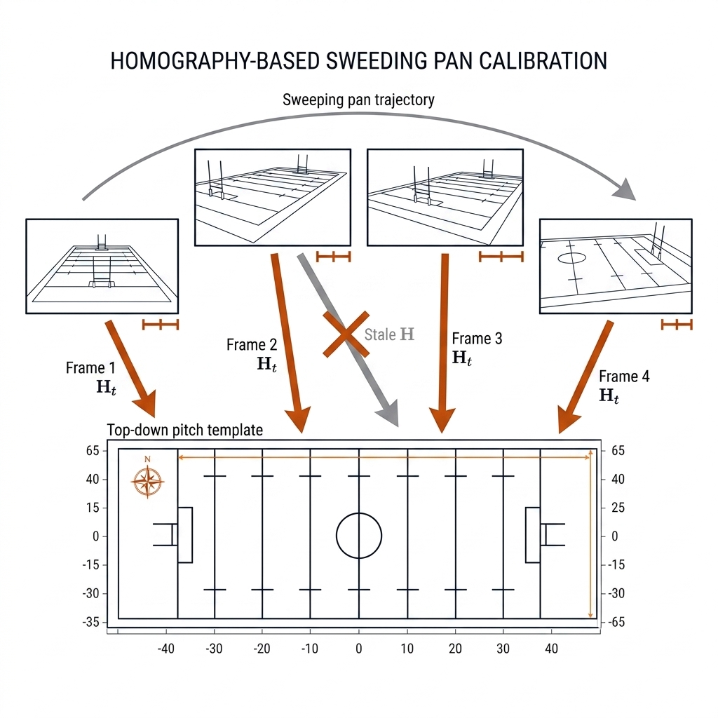
The pickleball broadcast case shows the mildest version of the loop: the court is static, only the camera moves. Between rallies the director pans from a wide court view to a player close-up; each pan invalidates the previous homography, so the pipeline re-estimates H at every frame during the sweep — but because the court is planar and small, the re-solve is well-conditioned whenever the kitchen line, a baseline, and one sideline are visible. Per-pan re-estimation on pickleball is nearly a solved problem at E11's 98.4% valid rate.
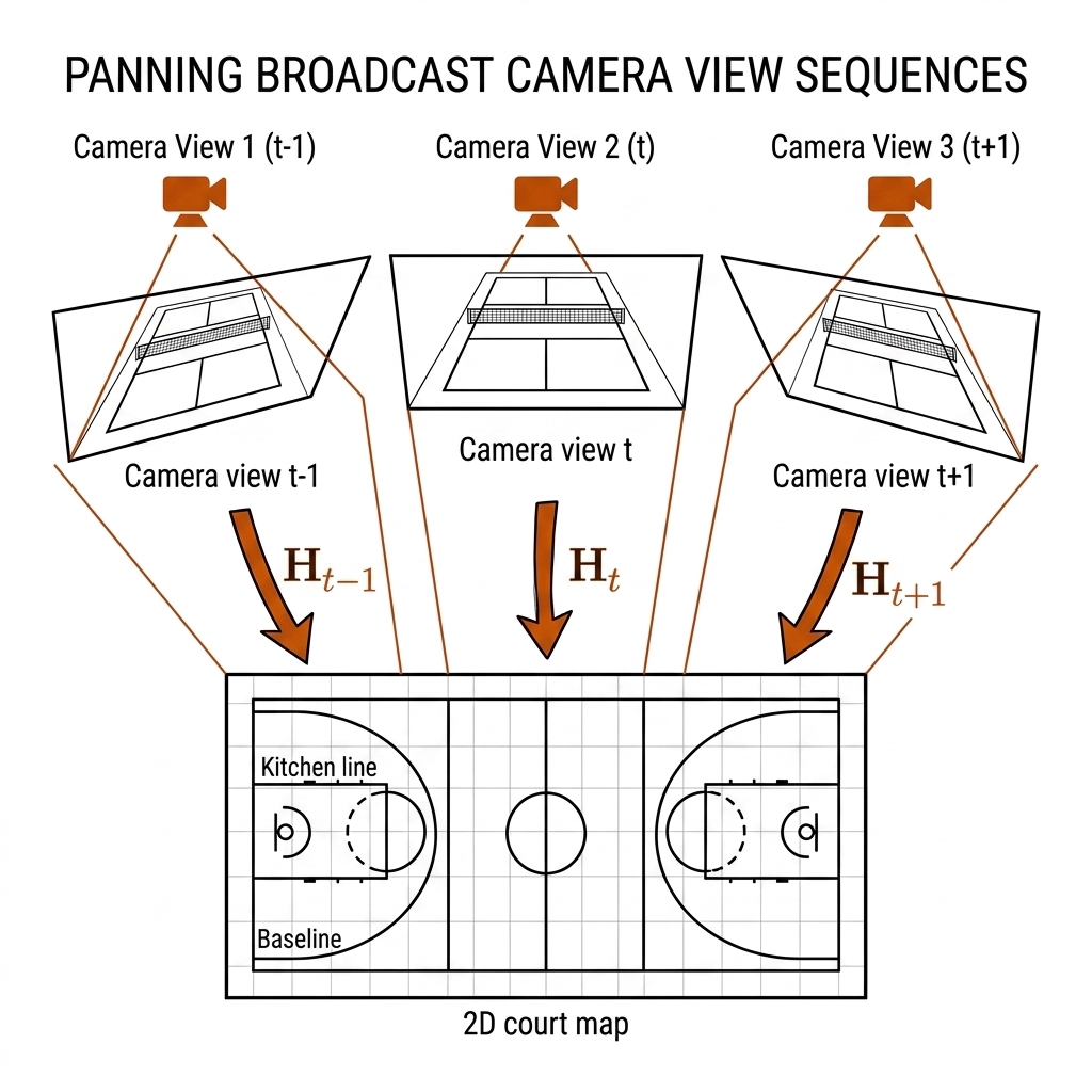
The rugby broadcast case is the same loop under hostile conditions: the pan is 100 m long instead of 13.41 m wide, the zoom range is wider, and the line evidence per frame is sparser and more occluded. Nothing about the architecture changes; everything about the valid-frame rate and the RMSE does. That is why the honest unit of comparison is not RMSE alone but valid_frames% at a stated RMSE (§7.8).
7.3 Measured Camera Regime (W2.2 Lab)
How much motion does a real broadcast clip actually contain? Our lab sampled dense optical flow over 701 frames of the nrl-001 clip and measured corner-level drift per frame:
| Drift Statistic | Value |
|---|---|
| Mean drift | 7.97 px/frame |
| Median drift | 4.86 px/frame |
| p90 drift | 21.24 px/frame |
| Max drift | 29.9 px/frame |
| Frames >1px | 73.0% |
| Frames >5px | 49.1% |
Two drift numbers coexist in this book and they measure different things — keep them straight. E08's tracker-level drift (median 0.0, p90 1.98, max 9.76 px/frame) is how fast player boxes move because of the camera, which is what the Kalman filter feels. The C07 lab numbers above are corner-level optical flow, which is what a homography feels. A homography is exquisitely sensitive to the tail: a 21 px/frame pan moves a pitch-line intersection by tens of pixels between frames, and the single-H reprojection error scales with it directly.
Nearly half the clip exceeds 5 px/frame of flow-level drift — yet the tracker-level median was 0.0. The tail is where panning and zooming live, and the single-H assumption fails there. The honest conclusion: a fixed homography is valid for maybe half of a rugby broadcast; the rest needs per-frame work.
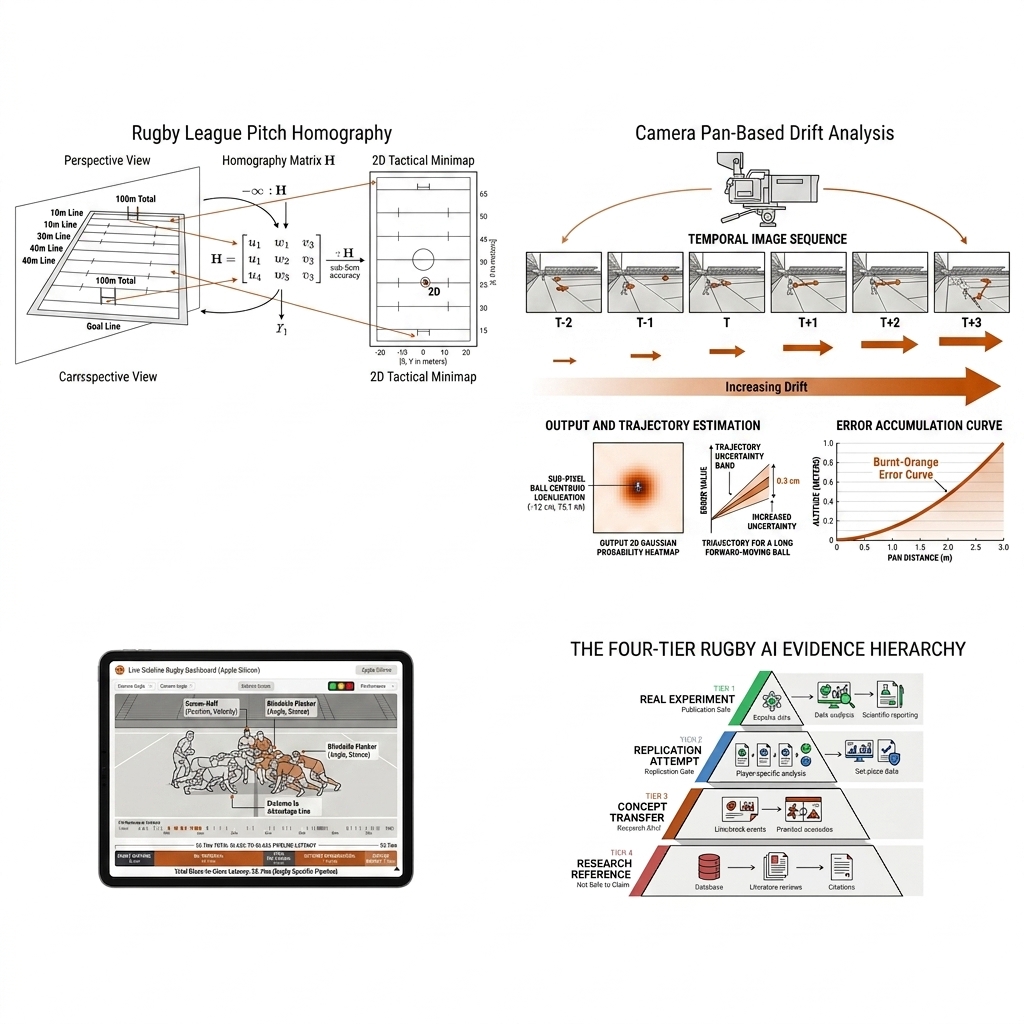
The pickleball broadcast regime is gentler in distance but identical in structure. A full-court pan covers 13.41 m instead of 100 m, so absolute drift per frame is smaller at the same angular speed — but the broadcast habit of zooming on the serve hits the weakness similarity models cannot reach: changing focal length. A 2× serve zoom on a pickleball broadcast changes the projective map as surely as a rugby zoom into a ruck, and no (tx, ty, θ, s) fit will express it. Distance is the rugby problem; focal change is everyone's problem.
7.4 Line Evidence: The Calibration Anchor
Per-frame calibration needs per-frame lines. Our lab ran classical Canny+Hough detection on 6 extracted frames of the nrl-001 clip as a cheap prior:
| Frame | Hough lines | Near-horizontal | Verdict |
|---|---|---|---|
| nrl-001-frame-01 | 8 | 7 | calibratable |
| nrl-001-frame-02 | 17 | 2 | calibratable (marginal) |
| nrl-001-frame-03 | 13 | 12 | calibratable |
| nrl-001-frame-04 | 10 | 10 | calibratable |
| nrl-001-frame-05 | 20 | 20 | calibratable |
| nrl-001-frame-06 | 4 | 4 | calibratable (minimum) |
The lesson: pitch-space calibration needs stable line correspondences; fewer than 2 near-horizontal lines = an ill-conditioned homography, and the pipeline must carry the previous H_t forward and flag the frame rather than fit garbage. Six of six frames were calibratable here, but frame-02's 2 usable lines are one occlusion away from failure, and these frames were selected to be open-play views — the tackle close-ups that dominate a broadcast's back half were not in the sample. Treat this table as an upper bound on classical line evidence, not a guarantee.
The sport contrast matters for method choice. Pickleball courts are line-rich and high-contrast: white paint on blue or green acrylic, seven lines in a 13.41 × 6.10 m rectangle, rarely more than four players to occlude them. Canny+Hough genuinely works there — that is C06's fixed-court recipe. Rugby league breaks every one of those assumptions: 24 bodies in a ruck hide the transverse lines, LED ad boards inject high-contrast moving edges that read as lines, shadow bands cross the pitch in afternoon games, and rain repaints the grass a colour the white-line mask was never trained on. Production rugby calibration needs the deep segment/keypoint detectors (TVCalib, roboflow/sports-style YOLO keypoint heads), with Hough retained as a sanity-check prior, not the solver.
The 2026 frontier (Theiner et al., CVSports best paper) handles the residual cases with joint registration + lens distortion modeling and a minimal point-on-segment annotation protocol — the successor to the TVCalib line, and the method to watch if your footage comes from action cameras rather than broadcast gantries.
7.5 The Rugby Template: Anchoring to Reality
Per-frame H_t is only as good as the thing it anchors to. The rugby league template is the 100 × 68 m field of play plus in-goals (6–11 m deep; a 116 × 68 m design plane covers the nominal case), and its markings are the calibration inventory:
| Element | Spec | Calibration value |
|---|---|---|
| Transverse lines | Every 10 m: 10/20/30/40 m + halfway | The ruler — any two visible lines + known spacing disambiguate zoom |
| 40 m lines | Often painted red (40/20 rule) | Colour cue for line-ID matching |
| Line width | 15 cm | The tolerance floor — sub-15 cm RMSE claims are inside the paint |
| Scrum markers | 10 m and 20 m in from each touchline | Extra keypoints on the near side |
| Goal posts | 5.5 m apart, crossbar 3 m | Post bases are high-value vertical keypoints |
| Touchline media line | 1.5 m outside touch | Trap — looks like a marking, must be excluded from the template |
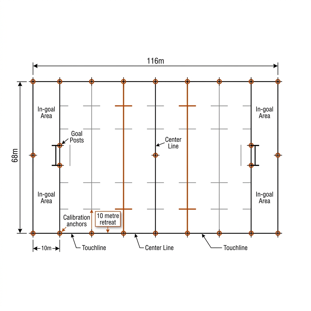
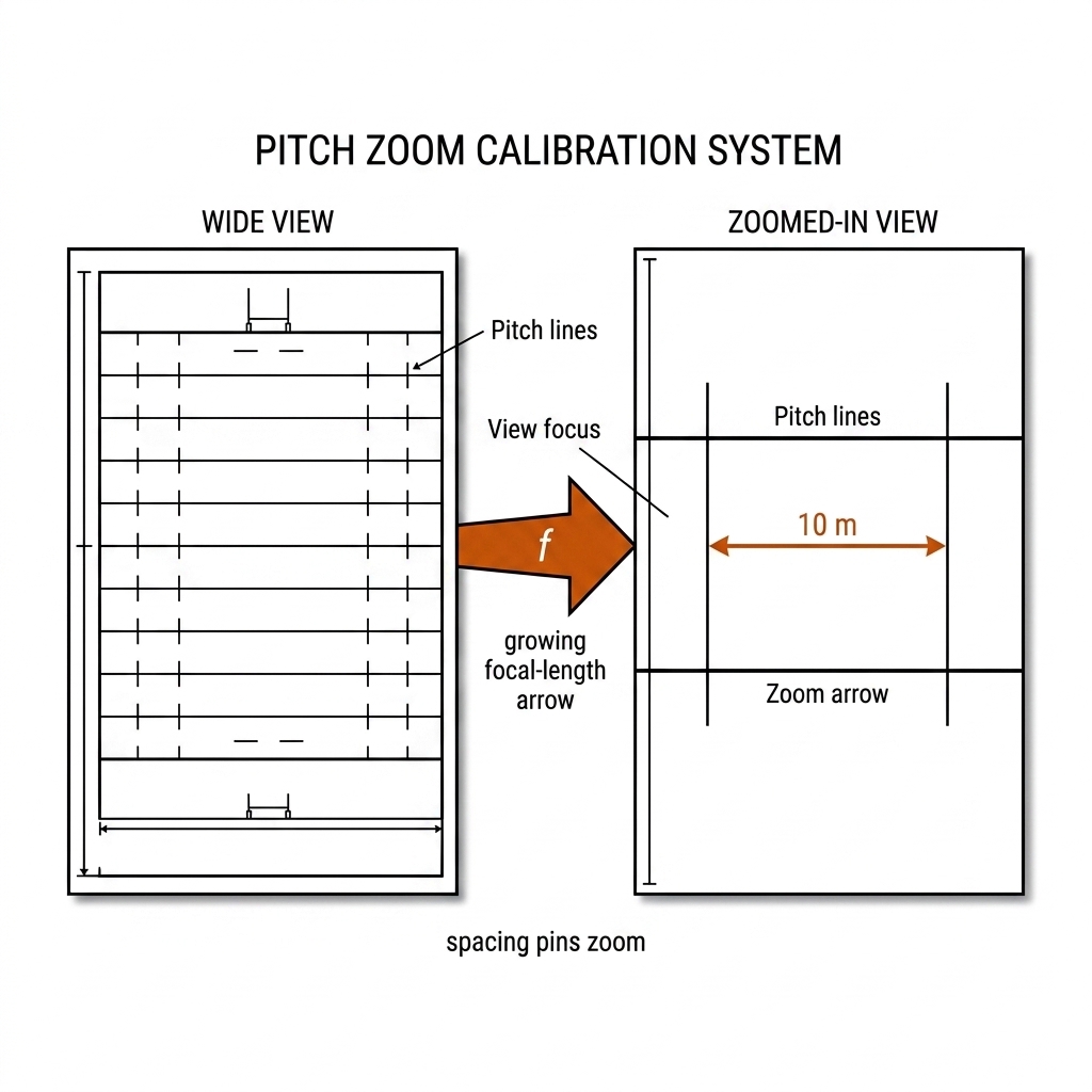
Zoom disambiguation deserves emphasis because it is the failure similarity models cannot fix. When focal length changes, everything scales — but the 10 m spacing between transverse lines is a known physical distance, so two visible lines plus their spacing pin the scale absolutely. This is why the line inventory, not corner keypoints alone, is the rugby calibration asset. The pickleball template plays the same role at smaller scale: the kitchen line sits exactly 2.13 m from the net and the baselines 6.71 m apart, so a serve-zoom frame that shows only the kitchen line and one baseline is still fully solvable. Four corners suffice for the fixed court (C06); broadcast needs the full line inventory because any given zoomed frame sees only a subset of it.
The two pitch-space payoffs for rugby analytics are the 10 m retreat check — the distance from the play-the-ball point to the defensive line, measurable only in pitch space — and the 40/20 line call. The pickleball equivalent is kitchen-fault adjudication: a foot on the kitchen line during a volley is a court-space measurement no image-space method can produce from a panning camera. Both sports monetize the same capability: metres, not pixels.
7.6 Cut Detection: The Missing Gate
A broadcast cut is not a calibration problem — it is a state reset. No frame-to-frame relation exists across a cut, so the LK flow prior, the GMC estimate, and the Kalman motion prior all become garbage simultaneously, and estimateAffinePartial2D will still happily return a RANSAC "fit" across the boundary if you let it. The pipeline contract:
- Cut gate runs BEFORE calibration (PySceneDetect BSD-3 CPU, or TransNetV2 via the MIT PyTorch port).
- On cut: invalidate the LK flow prior and the Kalman motion prior.
- Cold-start H_t from the first stable lines of the new shot.
- On gradual transitions (dissolves, wipes): mark frames low-confidence and let the §7.8 validator demote them rather than fit through them.
The sport-specific texture is fast cuts vs slow pans, and the two sports load different hazards. Rugby league highlights — the E14 footage — are cut-dense: a stinger wipe into an instant replay, a cut to the crowd, a cut back to a different gantry angle, several per minute. The dominant failure is the ungated cut: cold-start frequency is high, and false positives come from replay wipes and animated scorebugs, so the detector threshold stays conservative and the calibration validator is the second line of defence. Pickleball coverage is the opposite texture: rallies run long and uncut, the camera slow-pans and serve-zooms within a single shot, and cuts cluster between rallies. There the dominant hazard is not the cut but the slow pan — motion gentle enough that GMC and the H_t temporal prior keep producing plausible-looking answers while quietly drifting off the court. Slow pans fail softly; cuts fail loudly. A pipeline tuned for one hazard will miss the other.
Detection itself is solved and cheap — PySceneDetect's content detector is pure CPU and fast; TransNetV2's 3D-CNN handles the dissolves and wipes that heuristics miss. The engineering is the integration contract above, not the detector choice.
7.7 Repo Landscape and the GPL Trap
Every serious open calibration method in 2026 is soccer-first; both of this book's sports inherit from that lineage. The landscape, with the license column first because it decides what you may ship:
| Method | License | Status | Use for this book |
|---|---|---|---|
| sn-calibration (SoccerNet) | NO LICENSE | Reference dataset + Acc@5×completeness protocol | Cite, don't vendor |
| TVCalib (WACV 2023) | MIT | Dormant since 2024-04, but usable | Conceptual template for the E11-style loop (pickleball-measured) |
| PnLCalib (CVIU 2026) | GPL-2.0 | Strongest open solver (points + lines) | Evaluation-only for a commercial repo — copyleft contamination is a legal failure mode, not a technical one |
| roboflow/sports | MIT | Very active (2026-08) | The book's shipped recipe — swap the soccer template for §7.5's rugby template or the pickleball court |
| Theiner 2026 | code [verify] | The frontier; joint registration + lens distortion | Watch for consumer/action-cam footage (pickleball rec play) |
The GPL trap is worth naming plainly: PnLCalib is the strongest open solver and GPL-2.0, so vendoring it makes your whole pipeline a derivative work. The MIT path — the roboflow/sports keypoint-head recipe with a sport-appropriate template — is measurably good enough (E11: 98.4% valid at 4.65 cm on pickleball PTZ) and legally clean. Evaluate the GPL methods to know what the ceiling looks like; ship the MIT ones.
7.8 Confidence Metrics: valid_frames% Is the SLA
Report per-frame calibration as valid_frames% alongside RMSE, never alone. 100% valid at 40 cm RMSE is worse than 98.4% at 4.65 cm; the first number without the second is marketing. The measured anchors: E11's 98.4% valid at 4.65 cm was TVCalib-style calibration on pickleball PTZ; rugby broadcast will be lower — sparser lines, heavier occlusion — and must be measured, not assumed.
The supporting metrics, in order of operational value:
- Markings per frame — the leading indicator. E11 averaged 12.4 keypoints/frame on pickleball; fewer than 4 visible markings ≈ an unsolvable frame, and the honest move is to skip it, not fit it.
- Reprojection RMSE in cm — template markings reprojected into the frame. Accuracy when valid. Remember the 15 cm paint floor: sub-paint precision claims are noise on rugby.
- Acc@5 × completeness (SoccerNet protocol) and Jaccard over segments (Theiner protocol) — the benchmark metrics when you have labels, and the only way to compare against published soccer numbers.
- Parameter plausibility — recovered focal, tilt, and pan must sit inside physical broadcast ranges; a RANSAC fit to the wrong lines often fails this check even when reprojection looks fine.
- Downstream fragmentation — unique IDs and median track length after register-then-track. E14's 295 / 0.96 s baseline is the number a coach actually feels; everything above is instrumentation for improving it.
Report the failure histogram too — occlusion vs zoom vs cut — because the mitigations differ (§7.9), and a single valid% hides which lever to pull. For pickleball the dominant failure will be serve-zoom frames; for rugby, occluded rucks and heavy zoom. Different histograms, different fixes.
7.9 The Limits Table
GMC is an estimate, per-frame H_t is an estimate of a better kind, and both fail in enumerable ways. The honest table, with the sport that feels each failure most:
| Failure mode | Mechanism | Felt most in | Mitigation |
|---|---|---|---|
| Player occlusion of lines | Up to 24 persons/frame in rucks (E08, measured) | Rugby | Param-Kalman carry-forward ≤ N frames; valid% absorbs the drop |
| Heavy zoom / central views | Few or zero line intersections visible | Both (rugby tackle shots; pickleball serve zoom) | Circle/arc features (Magera 2025); parameter prior; skip frame |
| LED ad boards | High-contrast moving edges read as lines | Rugby | Mask board regions; colour-gated line detection (paint ≠ pixels) |
| Scorebugs / watermarks | Opaque overlays occlude anchor regions | Both | Static overlay masks per broadcaster; exclude from validation |
| Lens distortion | Consumer/action cams bend straight lines | Pickleball (rec-play footage) | Joint distortion solve (Theiner 2026) or undistort first from rig metadata |
| Whip-pan motion blur | 29.9 px/frame max drift smears markings | Rugby | Drop the frame; rely on smoothing; never force a solve |
| Cuts / wipes / replays | No frame-to-frame relation | Rugby highlights | §7.6 cut gate before anything else |
| Wet weather / repainted lines | Contrast loss, non-standard paint | Rugby (outdoor); rare for indoor pickleball | Training augmentation; classical fallback degrades first |
| GPL-2.0 solvers | Copyleft contamination | Both | Evaluate/cite PnLCalib; ship the MIT path |
| No rugby training data | All pretrained models are soccer-first | Rugby | §7.10 fine-tune on ~100 annotated nrl-001 frames |
The pattern across all ten: the calibrated frame count — not the model — is the production bottleneck. Every mitigation above is a way to spend the valid-frame budget honestly rather than a way to make the problem disappear.
7.9b The 10 Use Cases: Broadcast Calibration Applied
The use cases below are the applied bridge from the calibration machinery above to the two sports. They follow three tracks: Track A — Modelling the Camera (UC 01–03), Track B — GMC in Practice (UC 04–07), and Track C — Operations & Honest Measurement (UC 08–10). Each case states the practical problem, the mechanism with its math, and carries its evidence label — measured (E-number), source-backed (paper or verified repo), or [verify] where the lab has not run it.
Track A: Modelling the Camera (UC 01–03)
UC 01 — The Pan-Tilt-Zoom Camera Model
A broadcast director's camera never holds still, and the first question a calibration pipeline must answer on every frame is "what did the camera just do?" The mechanism: a gantry camera rotating about its optical centre induces an exact homography between frames, H = K·R_t·R_{t−1}⁻¹·K⁻¹; a zoom changes the focal length f inside K, which rewrites the projective map itself rather than rescaling it; roll is an in-plane rotation. The 4-DOF similarity that BoT-SORT's GMC fits (source-backed: tracker/gmc.py, verified at source) is the small-angle approximation of the rotation case and a crude stand-in for zoom. Payoff: choosing the right model per motion is the difference between a solvable frame and a silently wrong one.
UC 02 — Zoom Tracking via Known Line Spacing
A zoomed frame shows fewer markings, and a similarity's scale term cannot distinguish zoom from translation toward the plane — this is the failure mode no (tx, ty, θ, s) fit escapes. The mechanism: the template supplies absolute scale. Any two visible transverse lines plus their known physical spacing — 10 m apart on a rugby league field; baseline-to-kitchen 4.57 m on a pickleball court — pin the scale absolutely, so f is recovered inside the H_t solve rather than guessed (source-backed: §7.5 template; TVCalib solves pan/tilt/roll/focal jointly). Payoff: serve-zooms and tackle close-ups become calibratable frames instead of skipped ones.
UC 03 — Per-Pan Homography Re-estimation
Any H solved at the start of a pan is stale by mid-sweep: measured flow-level drift on nrl-001 reached 29.9 px/frame, so a pitch-line intersection moves tens of pixels within a second of panning. The mechanism is the per-frame loop — detect markings, match to the template, DLT + RANSAC solve, validate by reprojection RMSE — then Kalman-smooth the camera parameters (pan, tilt, roll, f), never the raw H entries, because element-wise filtering mixes projective terms and produces matrices that are not homographies of any real camera. Measured (E11): 98.4% valid frames at 4.65 cm RMSE, 11.2 ms/frame against a 40 ms broadcast budget. Payoff: no drift chain, and every frame carries its own checkable error — the SLA downstream analytics can trust.
Track B: GMC in Practice (UC 04–07)
UC 04 — GMC for Pickleball Broadcast
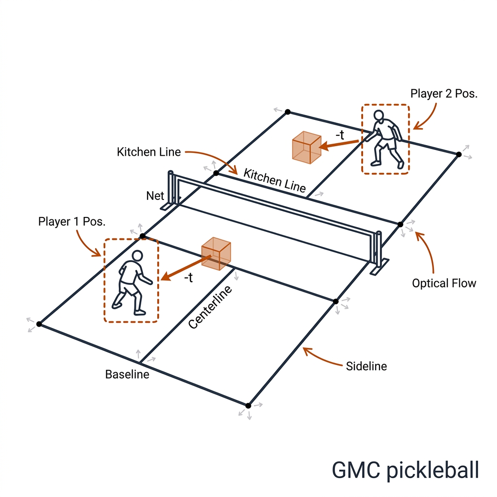
Rec-play and high-mast pickleball footage pans between rallies and zooms on the serve, breaking chapter 6's fixed-camera assumption. The mechanism is the same goodFeaturesToTrack → LK flow → estimateAffinePartial2D similarity pipeline; on a small, line-rich court with at most four players, the background consensus is strong and foreground contamination is low — the friendly case for GMC. Honest label [verify]: E14's GMC numbers are measured on rugby broadcast; pickleball broadcast GMC is not yet measured in the lab, and the fixed-camera E09 bake-off (ByteTrack 26 IDs → BoT-SORT 6, HOTA 0.642 → 0.814, measured) shows appearance ReID is the bigger lever while the camera holds still. Payoff: a cheap stabilization layer that ships free inside BoT-SORT (MIT) — as long as nobody mistakes its output for a calibrated view.
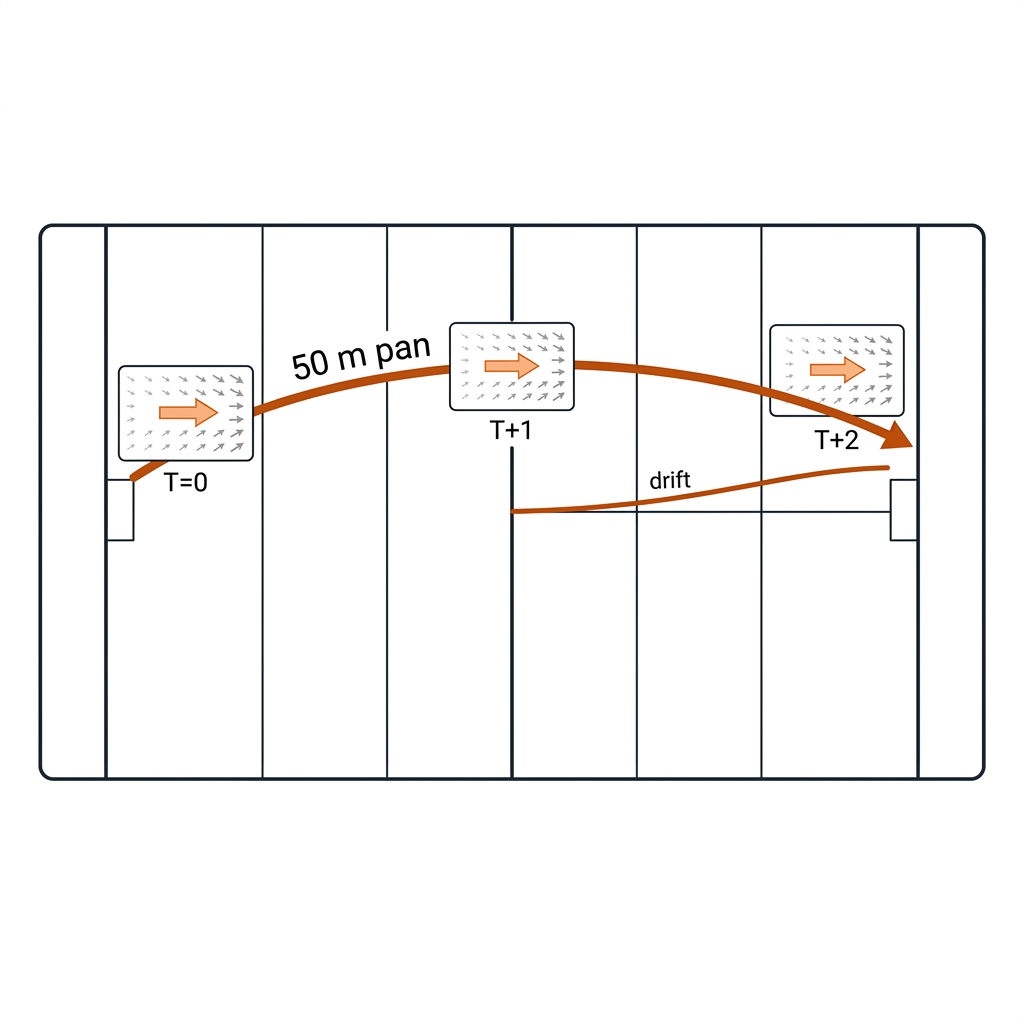
UC 05 — GMC for Rugby Broadcast: The 50 m Pan
The main gantry sweeps with every line break — 50 m pans are routine, and the E14 clip is exactly this regime. The mechanism, measured: GMC-framewarp bought +3.1% fewer unique IDs (295→286) with median track length 0.96→1.08 s; GMC-boxshift went backwards at −3.7% (306 IDs). The four caps from §7.1 bind here: mild median motion (tracker-level median drift 0.0 px/frame, E08 measured), the homography-vs-similarity model mismatch, translation-only downstream use, and foreground contamination from 13.2 detected persons per frame. Payoff: keep GMC inside the tracker when it is free; never present it as calibration — the metres come from H_t.
UC 06 — Athlete Masking for GMC (feeds from Chapter 10, UC 20)
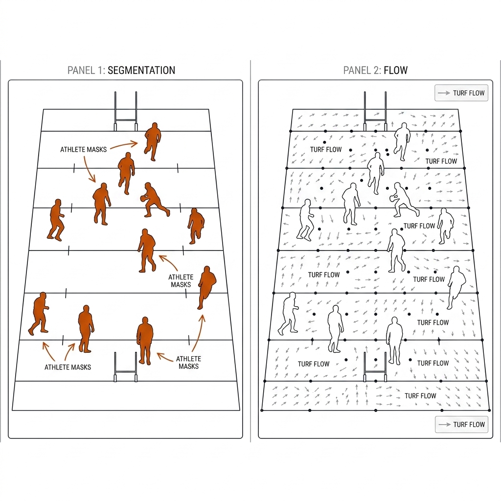
LK corners land on moving players; in ruck phases up to 24 bodies per frame (E08, measured) make the "background" the minority class, and RANSAC's consensus fit degrades exactly where IoU association is tightest — the book's working hypothesis for boxshift's −3.7% [book hypothesis; E14 did not ablate this]. The mechanism arrives from chapter 10's UC 20: SAM 2 binary athlete masks zero out the movers, the flow field is computed on static turf and line features only, and the similarity fit sees pure camera motion. Payoff: a structured error source removed at the tracker's most sensitive point, for the cost of masks the pipeline already computes.
UC 07 — The Drift Problem (The Honest Failure)
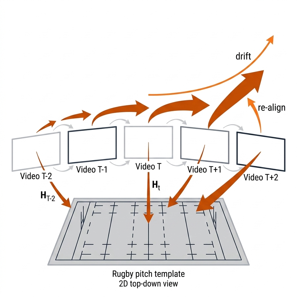
GMC anchors each frame to the previous frame, and nothing in the chain anchors to reality: the chained estimate H_chain = ∏ H_{t,t−1} accumulates every hop's RANSAC residual, the chain cannot detect its own accumulated error, and validity is unverifiable frame by frame. This is the structural failure per-frame H_t eliminates — independent solves against a fixed template, each carrying its own reprojection error. The measured contrast: GMC's best arm gained 3.1% on nrl-001 while E11's per-frame registration held 98.4% of frames at 4.65 cm under PTZ. Payoff: the honest SLA is valid_frames% at a stated RMSE — never stabilization smoothness.
Track C: Operations & Honest Measurement (UC 08–10)
UC 08 — Camera Cut Handling
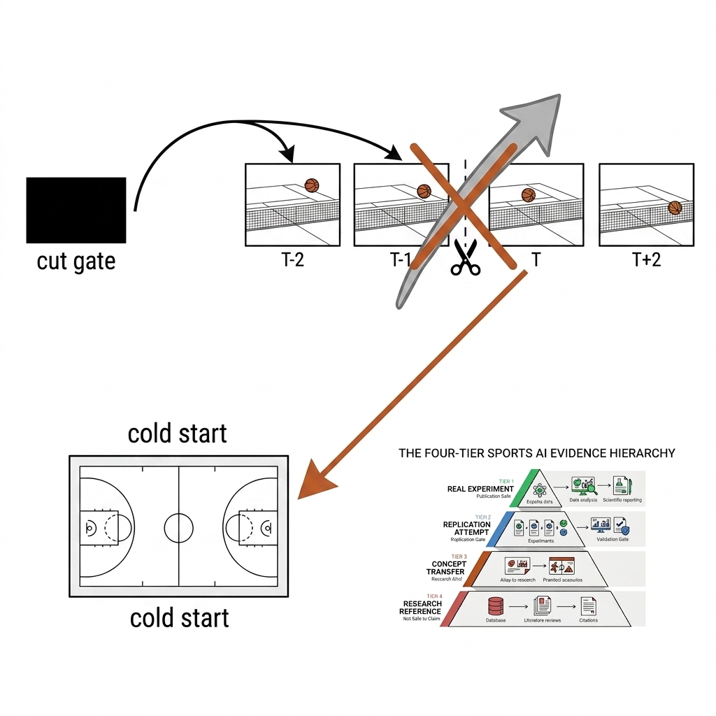
A cut is not a motion — no frame-to-frame relation exists across one, and estimateAffinePartial2D will still return a RANSAC "fit" across the boundary if ungated. The mechanism: a shot-boundary gate runs before calibration (PySceneDetect, BSD-3, pure CPU; or TransNetV2 via the MIT PyTorch port for the dissolves and wipes heuristics miss — both source-backed). On a cut, the pipeline invalidates the LK prior and the Kalman camera prior and cold-starts H_t from the new shot's first stable lines; gradual transitions are marked low-confidence and demoted by the §7.8 validator. [verify]: TransNetV2's published F1 is measured on general broadcast; the rugby-highlights false-positive rate on replay wipes and animated scorebugs is unmeasured — that is the E15 cut-gate audit. Payoff: the gate is cheap, and the ungated cut silently poisons every downstream number.
UC 09 — Static vs Broadcast: The Measured Tradeoff
When is the dynamic loop worth its cost? The mechanism is the side-by-side measurement: manual static homography at 3.82 cm, 100% valid, 0.02 ms/frame (E05) versus dynamic keypoint calibration at 4.65 cm, 98.4% valid, 11.2 ms/frame (E11) — 0.83 cm of accuracy and 1.6% of frames buy survival under PTZ. And the broadcast tax is mandatory once the camera moves: 49.1% of the nrl-001 sample exceeded 5 px/frame of flow-level drift (measured, C07 lab), so a single H is invalid on roughly half the frames of a real rugby broadcast. Payoff: spend the tax only where the camera actually moves — fixed rigs keep the cheaper, more accurate win.
UC 10 — The Broadcast-Quality Estimate: Is This Feed Calibratable?
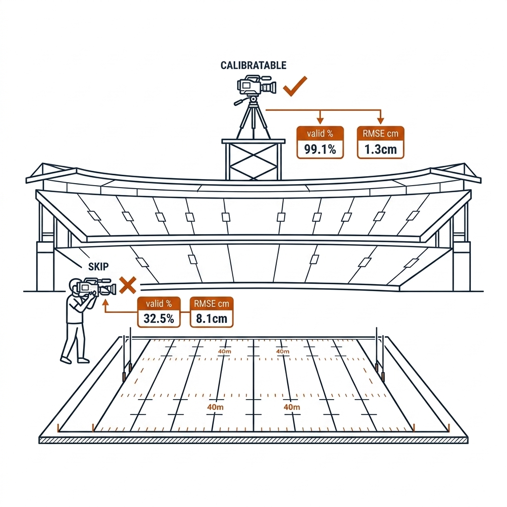
Before a club invests in broadcast analytics, the practical question is whether its feed can yield calibration-grade output at all — a high fixed gantry (the grandstand-level / high-tower positions, GL3/HT in broadcast camera plans) versus a low sideline handheld. The mechanism is a one-afternoon audit: sample dense optical flow for the drift profile (measured on nrl-001, 701 frames: mean 7.97, p90 21.24, max 29.9 px/frame) and run a line-evidence census (measured: 6/6 open-play frames calibratable by classical Hough, the marginal frame at 2 usable lines). High fixed gantries with the pitch in view pass; low moving handhelds fail the markings-per-frame floor of §7.8. [verify]: the camera-position → valid% mapping is a practitioner model; the audit instruments themselves are measured. Payoff: a cheap audit replaces a season-long failed deployment — and tells the coach which numbers to trust before a single model is trained.
7.9c What This Adds to the Pipeline
These ten use cases are not separate projects; they are one loop — gate, detect, solve, validate, smooth — applied to the two sports' camera regimes. They inherit chapter 6's fixed-camera calibration as the static arm (UC 09) and feed everything downstream that needs metres instead of pixels: chapter 9's tracking (UC 05's fragmentation numbers are the E14 baseline register-then-track must beat, per the FieldMOT architecture), chapter 10's UC 20 athlete masks (the input to UC 06), chapter 11's pose foot-points reprojected through H_t, chapter 12's ball trajectory in pitch space, and chapter 14's multiview fusion, which treats each broadcast frame as a moving camera with a per-frame pose. The pitch-space payoffs — the 10 m retreat, 40/20 adjudication zones, kitchen-fault measurement — are the features chapter 22's EPV and chapter 23's tactical models consume, and the live minimap chapter 28's cockpit renders. UC 10's audit is the gatekeeper for all of it: it decides, from a single afternoon of footage, whether a feed can support any of the chapters that follow.
7.10 What I Would Measure Next
- E15: annotate ~60–100 nrl-001 frames spanning zoom levels (transverse-line intersections, post bases, scrum markers against the §7.5 template) → Colab keypoint fine-tune on the rugby template via the MIT roboflow/sports recipe → per-frame H_t + parameter-Kalman smoothing (smooth pan/tilt/roll/focal, never raw H entries — element-wise filtering of H mixes projective terms and produces matrices that are not homographies of any real camera) → register-then-track vs E14 baseline. Targets: valid% ≥ 95, RMSE ≤ 10 cm (rugby tolerance is coarser than pickleball's 4.65 cm; the paint itself is 15 cm wide).
- Cut-gate audit: TransNetV2-PyTorch over the full nrl-001 GF broadcast, not the 30 s sample; measure reset behaviour and the rugby-specific false-positive rate on replay wipes and scorebugs.
- Pickleball side: per-pan re-solve evaluation on broadcast-style pb footage — pan the camera deliberately, measure how fast valid% recovers after each sweep and whether the serve-zoom frames are the dominant failure as predicted.
- Hypothesis to register: H_t beats GMC's +3.1% by a wide margin [verify by experiment — report whatever number actually lands], with the no-HOTA-without-labels gate carried forward from E14.
7.11 Sources
- E14 experiment:
experiments/e14-gmc/(baseline 295, boxshift -3.7%, framewarp +3.1%); E08 drift stats from its metrics.json; E09 tracker bake-off (HOTA 0.642→0.814) fromexperiments/e09-tracker-bakeoff/outputs/metrics.json; E05/E11 calibration numbers from their transcripts. - BoT-SORT GMC verified at source (MIT): github.com/NirAharon/BoT-SORT (
tracker/gmc.py, sparseOptFlow path); paper: arXiv 2206.14651. - Theiner, Müller-Budack, Ewerth — "Unified Sports Field Registration with Lens Distortion Modeling", CVPRW 2026, pp.10067-10076 (CVSports Best Paper): openaccess.thecvf.com.
- TVCalib (MIT, WACV 2023): arXiv 2207.11709; PnLCalib (GPL-2.0): arXiv 2404.08401; roboflow/sports (MIT): github.com/roboflow/sports; FieldMOT register-then-track (CVPRW 2025); Magera et al. central views: arXiv 2504.20052.
- Cut detection: PySceneDetect (BSD-3): github.com/Breakthrough/PySceneDetect; TransNetV2 (MIT): arXiv 2008.04838, PyTorch port github.com/allenday/transnetv2_pytorch.
- Rugby league geometry: NRL Laws of the Game (100 × 68 m field, in-goal 6–11 m, 10 m retreat, 40/20): nrl.com/operations/policy-documents.
- Lab:
lab/w2_lab_calibration_ii.py→experiments/c07-calib-ii/outputs/metrics.json(701-frame drift sampling, 6-frame Hough line audit).