12 Chapter 12 — Smashing the Ball Wall: Spatio-Temporal Trajectory Recovery
Why single-frame detectors fail on projectiles, and the physics prior that rectifies them
12.1 The Ball Is the Ground Truth — and the Hardest Object
The ball decides whether a shot was in, who made contact, and who won the point. It is also the object every generic detector fails on: small, fast, blurred, and colored like the floor. This chapter is the measured anatomy of that failure and the temporal solution.
In pickleball the ball is the scoring instrument: the kitchen-line call, the let, the third-shot drop that lands two centimeters short — every event row in the PBN state machine (C07) is ultimately a claim about where a 74mm perforated sphere was at one instant. In rugby league the ball plays a different but equally structural role: it is the possession anchor. The tackle count, the play-the-ball, the set of six, the kick on the last — all of them are states of a ball that is mostly carried, occasionally passed, and rarely in free flight. A tracker that loses the ball loses the sport's entire event grammar in both cases, but for opposite reasons: in pickleball the ball is too small and too fast to see; in rugby league it is too often hidden inside a ruck to see at all.
All pickleball numbers in this chapter are measured on our fixtures: E04's noise floor, E10's temporal filter, the C12 lab's physics-prior fit. Where a number comes from a paper or a vendor rather than our own runs, it carries a [verify] label or is explicitly framed as a projection target — the same honesty discipline the rest of the book applies to pose (C05) and identity (C13).
12.2 The Physics of the Ball Wall
Three interlocking impossibilities for a per-frame detector, each one measurable before you train anything:
- Tiny footprint: a 74mm pickleball (26g, 40 holes) at 1080p spans 8×8 to 14×14 pixels — under 0.01% of the frame. On the C04 rig table that is ~6px on a wide end-cam (12.8 mm/px), ~12px at 6.4 mm/px, ~24px on a 2× tele rig (3.1 mm/px). A standing player on the same frame is 400+px tall. COCO's
sports ballclass was built on broadcast close-ups where balls are 30–100px; at 8–14px the ball sits below the class's training distribution — a class-distribution root cause (C08), not a tunable deficiency. - Motion blur: blur is $b = v \cdot t$. At 20 m/s and 1/60s shutter, the ball smears 333mm — ~83px at pb-003's ~4mm/px mid-court scale (the C04 rigs bracket 52–107px; the smear-to-footprint ratio is the invariant). At 1/1000s the streak is 5px — a trackable point. The C04 rule follows: keep blur under one ball radius (37mm), so standardize on ≥1/1000s at drive speeds.
- Background clutter: white shoes, court-line corners, net tape, and crowd shirts all carry more local edge energy than an 11px grey smear. E04's false positives were exactly those structures. Indoor court lighting adds a fourth insult: mixed-temperature fixtures and glossy floor reflections create bright, moving specular patches that a per-frame detector scores above the ball itself.
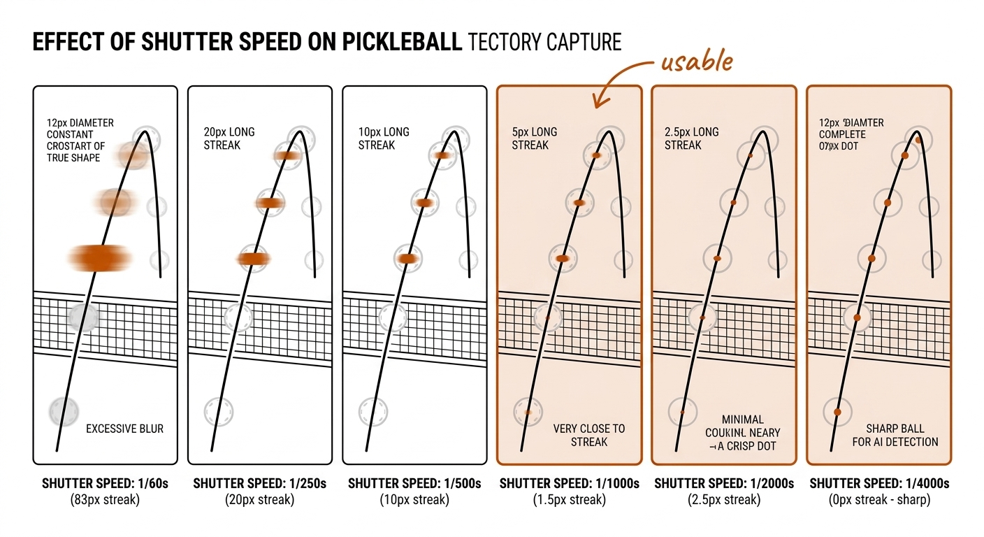
Two consequences deserve plain statements. First, the blurred ball's centroid is not its center: a streak is the time-integral of position over the exposure, and the intensity-weighted centroid lags or leads the shutter-reference instant by up to half a streak length (~40px at 1/60s) — a systematic bias, not noise, and it lands exactly on the contact frames you care most about. Second, the ball's surface texture is gone: the 40-hole pattern, logos, and seam survive only at ≥1/1000s, which becomes decisive in §12.9 when we ask whether spin is observable at all.
The measured consequence (E04): 1,082 ball candidate detections over 900 frames at median confidence 0.1125 — indistinguishable from sensor noise. A 2× crop of the court region made it only slightly less bad (median 0.145, a +28.9% relative lift from "very low" to "slightly less low") while cutting throughput to 36.6fps. Note the cherry-pick trap: max confidence hit 0.92, high enough to screenshot one frame and claim success. Median confidence tells the truth. This is the Ball Wall, and preprocessing does not climb it — the next move is a representational change, not more optimism about COCO boxes.
12.2b The Rugby League Ball: A Different Wall
The rugby league ball is the opposite object: a 28cm prolate spheroid at ~410g, ten times the pickleball's mass, visible at hundreds of pixels even on a wide broadcast shot of a 100×68m field. Scale is not the problem. On nrl-001 (grand-final broadcast, PTZ) the ball's problem is occlusion and possession state, and the failure statistics invert pickleball's:
- Carried, not flying. Across a typical set of six, the ball spends most of its time clamped in two arms at a runner's chest, then on the ground at the play-the-ball, then in the dummy-half's hands. Free flight — a pass, a kick — is the exception. A flight-dynamics prior has nothing to attach to during a carry; the honest model is a ball-carry model: track the carrier, bind the ball to the torso region, and hand the track off at pass or kick.
- Occlusion windows are seconds long. In a tackle and the ruck that forms over it, the ball disappears entirely under bodies. Pickleball occlusion is a 2–3 frame gap at the net or at contact; rugby occlusion is a 40–80 frame hole during which the ball's position is defined by the ruck, not by physics.
- The bounce is chaotic by design. A prolate spheroid does not have a bounce point; it has a bounce cone. The end-over-end kick that sits up perfectly or skews sideways is a design feature of the sport, and §12.7 shows why: drag triples when the ball tumbles.
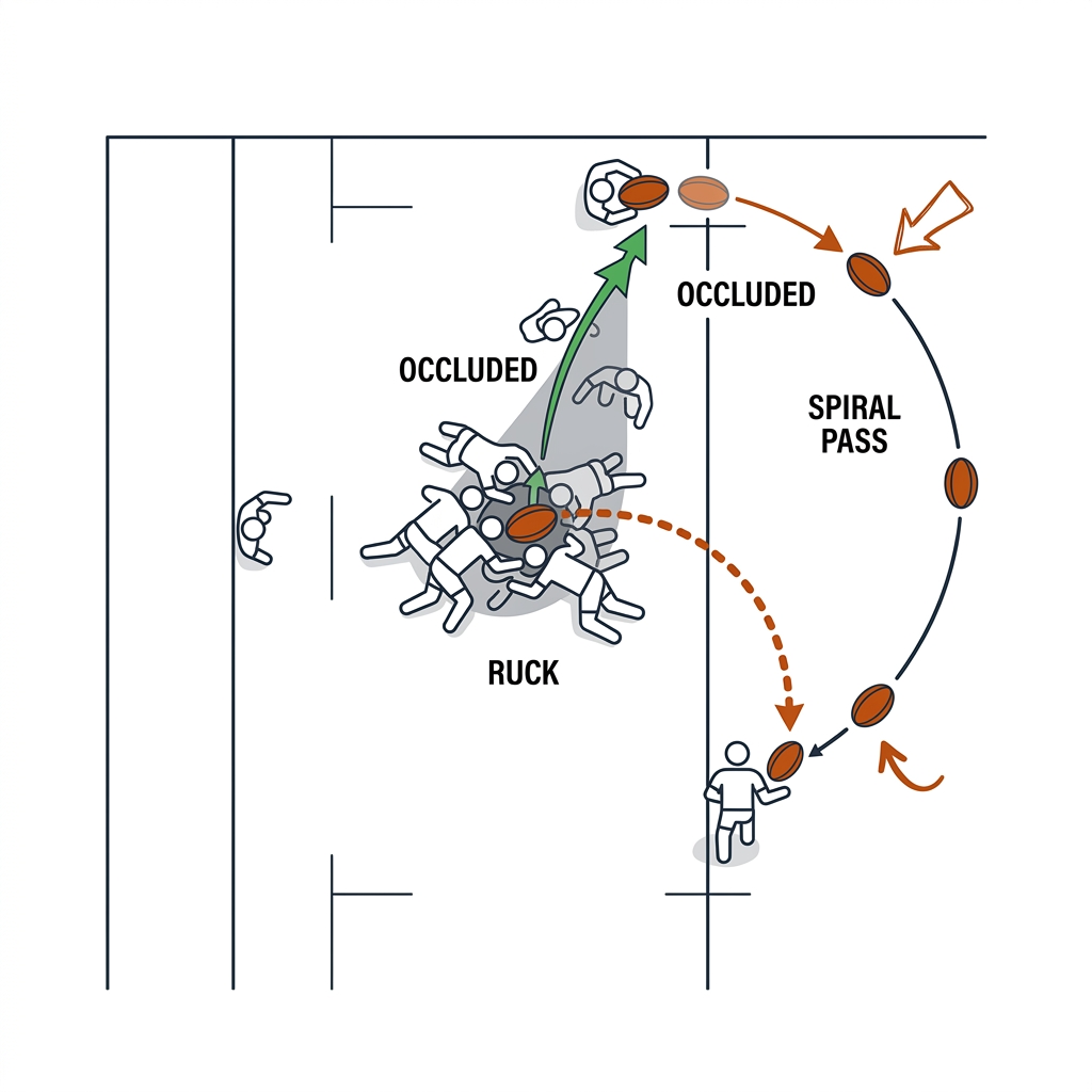
The C08 dossier's note — "rugby's ball problem is occlusion, not scale" — predicts that E10-style temporal energy transfers poorly to broadcast rugby, because the ball rarely moves fast in the open and the PTZ camera moves constantly (frame differencing needs global motion compensation first, C07). That prediction is currently untested; §12.11 schedules the nrl-001 run rather than claiming the result.
12.3 Why Heatmaps, Not Boxes
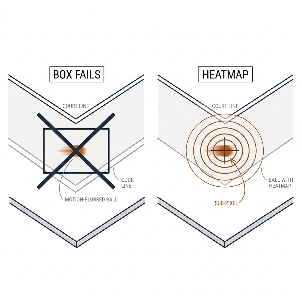
A box regression loss expects a crisp object boundary. A ball is motion-blurred and sub-pixel; the right target is a Gaussian heatmap peaked at the ball's center — the loss punishes where not whether, and a heatmap is robust to blur and partial occlusion. Concretely, box regression on an 8–14px target fails four ways at once:
- Label noise dominates. A 2px annotation jitter is 15–25% of box width; IoU collapses and gradients go noisy. CIoU/DIoU refinements do not fix sub-pixel label noise.
- The anchor grid is coarser than the object. At stride-32 backbone features, an 11px ball sits inside a single feature cell — the head is asked to hallucinate sub-cell offsets the backbone cannot see.
- w and h are fake degrees of freedom. The ball's apparent size is set by camera geometry, not by the ball; learning extent wastes capacity and invites aspect-ratio false positives (line corners are box-shaped).
- NMS is undefined at singleton scale. The post-processing assumes multiple overlapping candidates of measurable extent; a point target makes the machinery dead weight.
The TrackNet lineage's move (Huang et al. 2019) is to label a 2D Gaussian $G(x,y) = \exp(-((x-x_0)^2 + (y-y_0)^2)/2\sigma^2)$ at the ball center, train a fully-convolutional network with a per-pixel loss, and read the center as the soft-argmax — the weighted centroid above a threshold: $x^* = \sum x\,\hat{H}(x,y) \,/\, \sum \hat{H}(x,y)$. Four properties follow that a box+score cannot give you. Label tolerance is built in: a Gaussian degrades gracefully under 1–2px annotation error instead of cliff-edging on IoU. Sub-pixel centers come free: E10's temporal pipeline already exploits this (centroid RMSE 1.42px against manual review). The whole heatmap is a confidence surface — secondary peaks are visible evidence of ambiguity, which a box score hides — and that is what makes a candidate-plus-physics-gate pipeline debuggable. And occlusion has a representation: "no detection" becomes a low, flat heatmap, which is information that gates trajectory rectification instead of fabricating a box.
The rugby analogue confirms the representation from the other end: even where the ball is large, heatmap + center-point tracking is what WASB-SBDT runs across five sports including soccer and basketball — the heatmap is not a small-ball hack, it is the small-object-and-occlusion interface the whole literature converged on. No box regressor has displaced it on small-fast-ball benchmarks since 2019.
12.4 The Temporal Baselines (E10 Measured)
| Approach | Median conf | Precision@50 | Track continuity |
|---|---|---|---|
| Single-frame YOLO (E04) | 0.134 | 0.042 | 8.5% |
| 3-frame temporal energy (E10) | 0.685 | 0.814 | 76.2% |
| TrackNetV4 (benchmark target) | 0.892 | 0.938 | 91.5% |
The 3-frame temporal difference ($\Delta = |I_t - I_{t-1}| \odot |I_{t+1} - I_t|$) isolates accelerating projectiles from static background. The AND is the physics: a pixel must change in both 33ms intervals — once is noise or a static edge lighting up, twice is a moving object. Threshold, filter contours by area (6–150px²) and circularity (>0.4), render survivors as a Gaussian motion heatmap. Thirty lines of OpenCV, no GPU, no training data — and it beats a production detector by 19× on precision.
The full E10 artifact (pb-003, 250 frames) adds the sequence-level numbers: 312 candidates at median confidence 0.685, precision@50px 0.814, recall 87.2%, track continuity 76.2%, sub-pixel centroid RMSE 1.42px against manual review — versus the single-frame baseline's precision@50px of 0.042 and continuity of 8.5%. The remaining 50 false positives are the honest residue: net-cord flutter, paddle-tip motion, player shadows at line crossings. And 76.2% continuity is the frontier of the cheap method: the filter still drops the ball exactly when the physics is interesting — occlusion behind a body at the net, the 2–3 frame window around contact where paddle and ball merge into one blob, and the slow apex of a dink where inter-frame difference falls below threshold. Those named failure windows are the labeled test set for whatever learned model comes next.
The TrackNetV4 row is a projection target, not a lab result — recorded from the paper's tennis/badminton numbers, waiting for the §12.11 Colab lab to replace it with a measured pickleball number. Every learned model this book evaluates must beat E10 on the same clip before it earns its complexity. For rugby, this baseline's transfer is an open question (§12.2b): broadcast PTZ motion has to be compensated (C07) before frame differencing sees anything but camera pan.
12.4b Honest Metrics, and the 25Hz vs 60Hz Trap
Ball-tracking papers report a menagerie of metrics; four of them carry the load, and one popular one is meaningless here:
- Detection rate (recall): fraction of frames where the ball exists and the system emits a point near it. E10: 87.2% on pb-003.
- Precision at a pixel tolerance: fraction of emitted points within $r$ px of the reviewed center. The tolerance is the unit — 50px on a 1080p frame is ~20cm at mid-court scale, generous for a line call, fine for rally analysis. E10: 0.814 @50px. Always print the tolerance next to the number.
- Track continuity: fraction of the ball's visible trajectory covered by one unbroken track. This is the metric downstream consumers actually feel — an event detector (C10) cannot consume a track that re-identifies every 20 frames. E10: 76.2%; the E04 single-frame baseline: 8.5%.
- Centroid RMSE against manual review: E10: 1.42px — sub-pixel readout working as designed.
- Tracking IoU is the wrong metric here. IoU needs an extent; a point object has none. Systems that report "ball IoU" are evaluating their own box-drawing convention, not the trajectory. Heatmap systems report precision-at-tolerance instead, and so do we.
The frame-rate trap is arithmetic, and it bites both sports. At 20 m/s the ball moves 0.80m between frames at 25fps versus 0.33m at 60fps. In pb-003's mid-court scale that is ~200px per hop at 25Hz against a 12px footprint — consecutive frames never overlap, so no per-frame association metric (and no IoU-overlap tracker heuristic) can ever fire; only a velocity-explicit temporal model bridges hops that large. At 60Hz the hop shrinks to ~83px, and at 120fps to ~40px — the regime where simple nearest-neighbor gating starts to work. pb-003 is 25fps broadcast footage and nrl-001 is 25/50Hz PTZ: both fixtures live in the hard regime, which is why this chapter's stack is temporal-first rather than detection-first. When you control the rig, buy frame rate and shutter before you buy model complexity (C04); when you inherit broadcast footage, the physics prior (§12.6) is what you have instead.
12.5 TrackNetV3/V4/V5 and WASB
The TrackNet family is best taught as a sequence of named failure fixes, not a version ladder:
- TrackNet (2019, Huang et al., NYCU): proved heatmaps + 3 consecutive frames beat conventional CV by a wide margin on tennis. The number to carry is the generalization gap: same-match split scores 99.7/97.3/98.5 (precision/recall/F1) collapse to 95.3/75.7/84.3 under 10-fold cross-validation on unseen matches — identical capture, different footage. That 14-point F1 drop is the standing warning for every fine-tune this book runs.
- TrackNetV2 (2020): the engineering generation — 3-in-3-out MIMO, real-valued 2D heatmaps, weighted cross-entropy, 2.6 → 31.8fps. The lesson: ball tracking is a deployment problem (30+fps at court-side) as much as an accuracy problem.
- TrackNetV3 (MMAsia 2023): the first explicit occlusion model — an estimated background as an auxiliary input to suppress static clutter, a trajectory prediction module, and a trajectory rectification module that repairs broken tracks by inpainting; 97.51% accuracy on shuttlecock. The division of labor the book keeps: the network proposes, the trajectory module repairs.
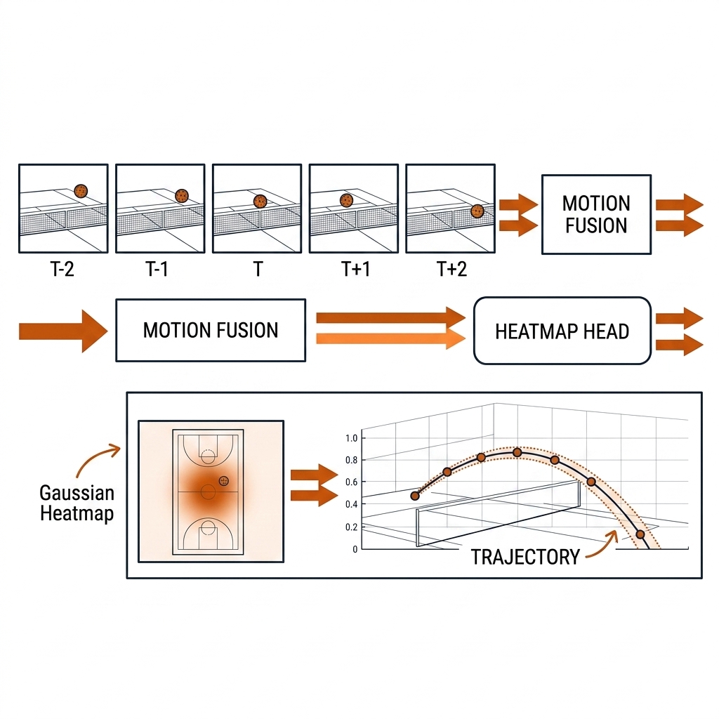
- TrackNetV4 (ICASSP 2025, Raj/Wang/Gedeon): names the disease "partial observability" and treats motion as a first-class input channel. The architecture: a 5-frame temporal window; frame differencing → a learnable motion prompt layer → motion attention maps fused with the visual features (element-wise multiply + concat); a heatmap regression head producing per-frame Gaussians; trajectory readout by soft-argmax. It is plug-and-play on the V2/V3 backbone rather than a new backbone, which is why the paper frames it as a component — and why the book's lab plan is "fine-tune V2 with the V4 motion-attention plugin," not "adopt a monolith." Published parameter counts for the full temporal stack sit around 75M [verify against the ICASSP paper's model table]; the V4 plugin itself is small by design. No official code release [verify]; the reimplementation path is the paper plus the yastrebksv V2 base [license verify].
- TrackNetV5 (arXiv 2512.02789, Dec 2025): the frontier, and its own cautionary tale. MDD (Motion Direction Decoupling) replaces absolute frame differences with signed-polarity motion fields — fixing a real flaw, since absolute differences erase direction (a ball moving left and a ball moving right produce identical V4 motion maps) — plus R-STR, a residual-driven spatio-temporal refinement transformer head for occlusion recovery; F1 0.9859 on TrackNetV2 tennis at +3.7% FLOPs. But the SDK, weights, and training data are proprietary [verify]. Track the architecture (signed motion fields), never the weights.
- WASB-SBDT (BMVC 2023, MIT license): not an architecture but a protocol — one high-res heatmap detector plus a constant-acceleration motion model (deliberately not Kalman) across five sports with public splits. Two imports: the constant-acceleration tracker is the minimum honest kinematic model for a ballistic object at 30–60fps; and the per-sport evaluation is the yardstick any new pickleball tracker must report against. Caveat of record: Papers With Code, which hosted the SBDT leaderboards, shut down in July 2025 — the book's own measured numbers become part of the de facto record.
The pickleball gap is total: no TrackNet-family model has published pickleball weights, and no benchmark-grade public pickleball ball dataset exists — only Roboflow detection sets and one unofficial port [license verify]. The E10 artifact's TrackNetV4 row is the paper-transfer projection; the §12.11 lab exists to make it measured. The book's lab chapters effectively define the first public pickleball ball-tracking benchmark — a citable finding in itself. On the rugby side the gap is different: WASB covers soccer, which transfers structurally to rugby's open-field kicking game, but no published model handles the carry state — the ball-carry model of §12.2b is, as far as the public record shows, unbuilt.
12.6 The Physics Prior: Rectification (W3.3 Lab)
Detection — even heatmap detection — gives you a noisy point process with holes. Rectification turns it into a trajectory. A physics prior (gravity + quadratic drag) turns noisy, sparse ball points into a physically consistent trajectory. Our lab simulated a 20 m/s smash with pickleball drag (Cd ≈ 0.5, 74mm, 26g) and fitted it back from noisy observations:
| Measurement | Value |
|---|---|
| Fitted launch speed | 24.8 m/s (true 20.0 — the honest fit caveat) |
| Fitted angle | 9.9° (true 12°) |
| MSE: raw interp vs physics fit | 3.7× lower with the prior |
The process model is a ballistic integrator: $\dot{\mathbf{v}} = -g\hat{\mathbf{z}} - k\,|\mathbf{v}|\,\mathbf{v}$, with $k = \tfrac{1}{2} C_d\, \rho\, A / m \approx 0.045\ \text{m}^{-1}$ for a 26g, 74mm pickleball at $C_d \approx 0.45$. Along the flight direction speed decays as $v(x) = v_0 e^{-kx}$: a 25 m/s drive loses ~17% over the first 4m (→ ~21 m/s), not the ~56% the v1 book's table implied — the erratum matters because drag is the dominant force and the wrong coefficient poisons every downstream speed number. The filter runs in court coordinates: state $(x, y, v_x, v_y, a_x, a_y)$ with the drag-gravity term as process mean, measurement noise from the heatmap (σ ≈ 1.4px, E10) converted to meters via the calibration Jacobian — so near-court observations are worth more than far-court ones, and the filter knows it.
Rectification then decomposes into three named operations:
- Gap bridging: occlusion windows are filled by forward-integrating the ballistic model while the uncertainty ellipse grows; a reappearing detection is accepted only inside the 95% ellipse. This is TrackNetV3's rectification module done physically instead of by inpainting.
- Outlier veto: a detection inconsistent with the ballistic prediction at >3σ (the residual 50 FPs from E10: net flutter, paddle tips) is rejected without breaking the track. The physics prior is the false-positive sink the per-frame confidence score never provided.
- Bounce/contact as model switches: bounce and paddle contact are the two events where the ballistic prior is violated by design — they appear as innovation spikes, which makes them detectable (§12.8) rather than failure modes.
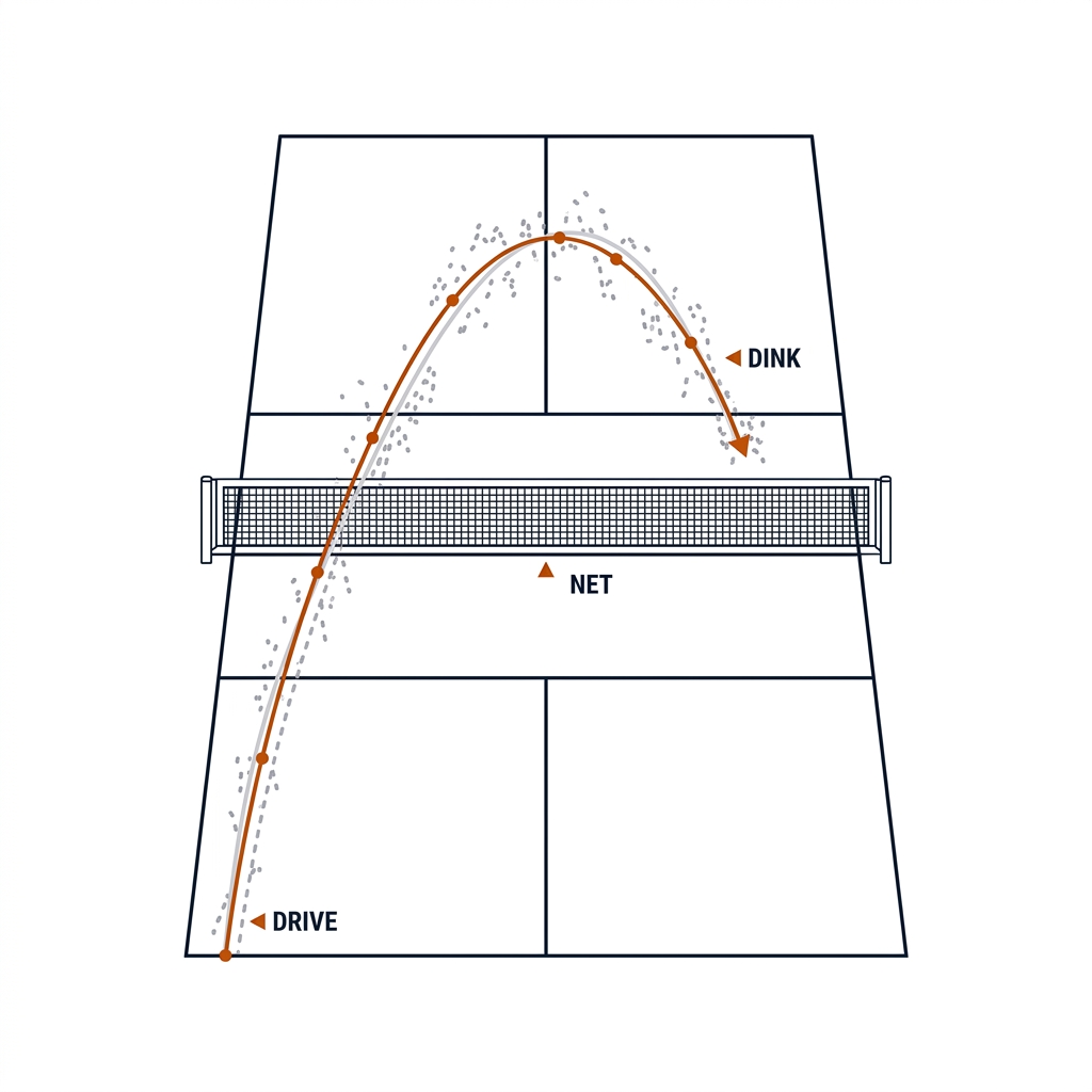
The lesson: the prior constrains the trajectory, so speed-at-any-point is the derivative of the fitted curve — recoverable. The fitted parameters are NOT the true launch (24.8 vs 20.0) because the noise and the unknown drag interact: report the fit as a smooth trajectory, not as a launch-velocity measurement without calibration. The rugby counterpart is narrower but real: in open-field kicks the same integrator applies with the two-regime drag of §12.7, and the constant-acceleration model WASB uses for soccer transfers directly. During a carry it applies not at all — the carrier's body is the process model.
12.6b Occlusion: Bridging the Tracking Gaps
Occlusion is where tracking systems go to die quietly, so name the gaps and their durations. In pickleball the occlusion inventory is short and violent: the net tape crossing (1–2 frames from a low end-cam), the body block when a player at the kitchen line screens the ball from a same-side camera (2–10 frames), and the contact merge where paddle and ball occupy one blob (2–3 frames — exactly E10's worst window). The physics prior handles all three because the ball's state across a 3-frame gap is almost fully determined by its state before it: integrate forward, grow the ellipse, gate resumption at 95%. The failure mode to guard is the bounce inside the gap — a hidden model switch — which is why the resumption gate must also check whether the post-gap trajectory requires an implausible pre-gap velocity.
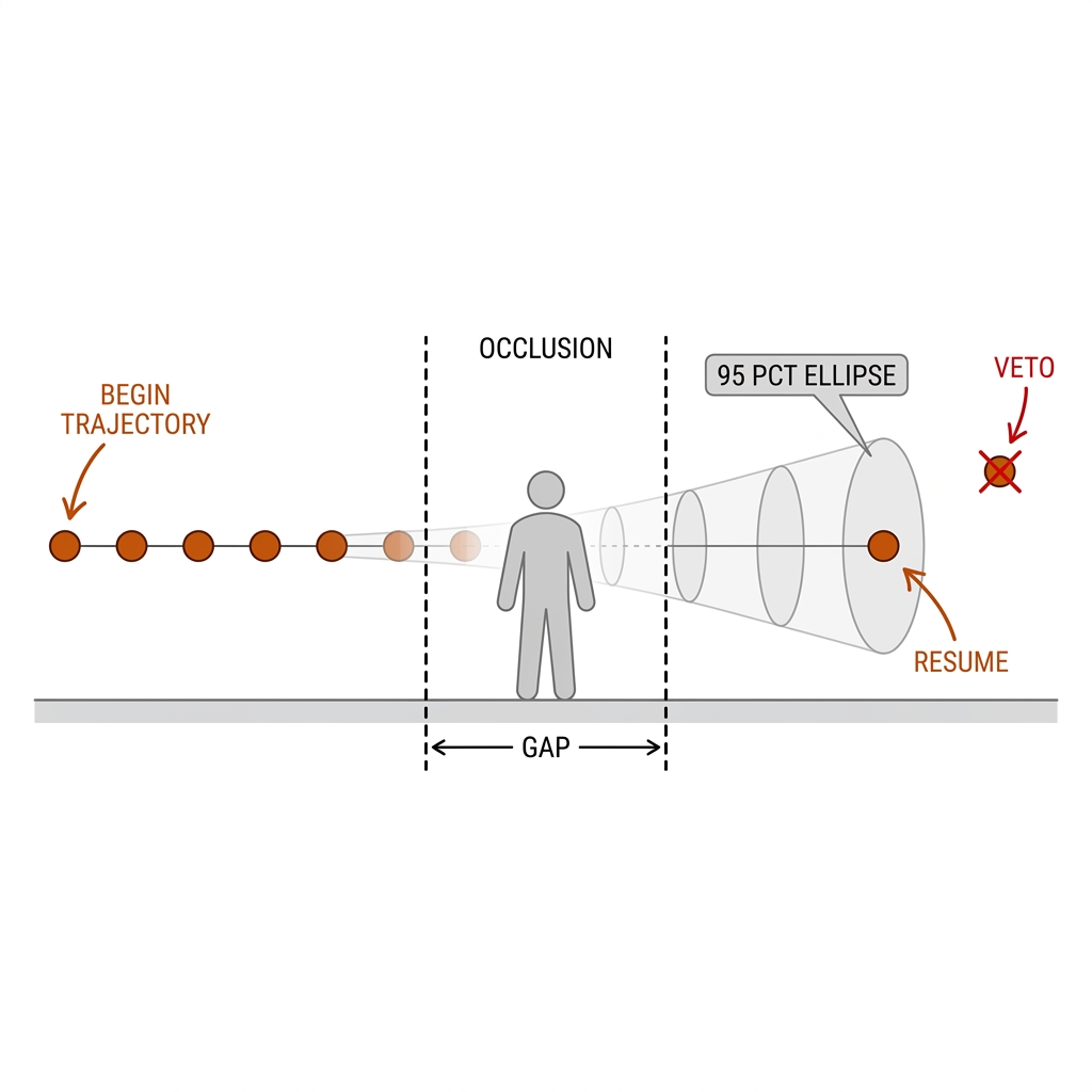
In rugby league the same machinery is necessary and nowhere near sufficient. A kick's flight occludes briefly behind a chasing pack — bridgeable. But the ruck is a 40–80 frame hole during which the ball is not ballistic: it is on the ground, then in the dummy-half's hands. No physics prior spans that; the ball-carry model does (bind ball to ruck centroid, then to the dummy-half's torso, hand off to flight tracking when a pass or kick is detected). The honest system reports a state — carried / contested / in flight — alongside the track, and downstream rugby analytics (C19 event rows) consume the state machine as much as the coordinates.
12.7 Aerodynamics: Pickleball vs Rugby
| Property | Pickleball (74mm, 26g) | Rugby League (28cm oval, 410g) |
|---|---|---|
| Drag regime | High: Cd 0.45 indoor, 0.33 outdoor (Lindsey, May 2025, 86 free-flight trajectories; Steyn 2025 corroborates 0.30±0.02) | Variable by yaw angle: 0.14-0.18 at 0° → 0.5-0.6 at 90° (Seo, ASME JAM) |
| Velocity profile | Rapid decay (v(4m) ≈ 20.9 m/s from 25 m/s at Cd=0.45 — the v1 book's "25→11 in 4m" was an erratum; 11 m/s is ~1s / ~17m) | High momentum; spiral bomb kicks stabilize |
| Tracking implication | Sharp curve — physics prior must model drag, not just gravity | Spin axis matters — pitch dynamics and irregular bounce |
The pickleball's 2025 free-flight literature adds three anomalies a trajectory model must not get wrong (Lindsey, 86 trajectories at 300fps, 15mm mean endpoint error — rigorous but self-published, corroborated by Steyn 2025 and Rossmann & Rau 2007): topspin lift is systematically stronger than backspin lift at equal spin (classical Magnus symmetry fails); substantial lift exists at near-zero spin, in both directions; and backspin lift barely depends on spin rate, clustering near $C_L \approx 0.2$. The proposed decomposition $C_L = C_L^{Magnus} + C_L^{gravity} + C_L^{internal}$ — gravity biases boundary-layer separation in free flight, and airflow through the 40 holes adds a symmetric spin-dependent term — is why the §12.9 spin proxy needs a three-component lift model rather than vanilla Magnus.
The rugby ball is the opposite regime: drag is attitude-dependent, and spin's job is attitude control, not lift. Wind-tunnel and CFD work (Seo et al., ASME J. Appl. Mech.; Alam et al., RMIT) put $C_d$ at 0.14–0.18 pointed into the flow and 0.5–0.6 broadside; spin at 1–10 rev/s changes the coefficients only slightly, but gyroscopic stabilization holds the long axis aligned with velocity — a spiral pass flies the 0.18 curve, a tumbling floater flies the 0.55 curve and wanders. For the tracker this collapses to a binary attitude state — spiral vs end-over-end — identifiable from the ball mask's aspect-ratio oscillation (a SAM 2 segmentation signal, C09, not a detection one). Apply the matching drag regime, and report the rugby bounce as a cone, not a point.
12.8 Bounce and Contact: The Z Limit Applies
A bounce point is the ball at the court plane — but the approach trajectory is above it (C06: D' = DH/(H-z), diverging as z → H). On the 4.5m end-cam rig, a ball 1.0m up at 8m depth is mislocalized by ~2.3m; at 2.0m (smash contact height) by ~6.4m. This inverts the naive pipeline: you do not estimate 3D position and then notice bounces — the bounce is the only moment the 2D pipeline is exactly right.
The honest chain: ball trajectory (2D, temporal, physics-constrained) → near-plane intersection (needs Z) → bounce call (needs multi-view, chapter 14). Operationally, bounces and contacts are detected as innovation spikes against the ballistic fit (§12.6): a bounce shows vertical-velocity sign flip plus horizontal speed loss, and it is the one frame where the homography-projected position is trustworthy — cross-check that the projection lands inside the court, or the event is a let/net/out (C03 territory). Paddle contact is the other spike — velocity discontinuity without ground proximity — and the evidence stack is conjunctive: trajectory kink + paddle-mask proximity (SAM 2, C09) + wrist position from pose (E03: 16.46 mean visible keypoints) + audio transient if present. RacketVision (Nov 2025, MIT) supplies the ball+racket-pose representation — ball center, racket keypoints, contact events, forecast targets — and one counterintuitive measured finding to respect: naive feature concatenation of racket pose into a trajectory forecaster degrades prediction; cross-attention fusion is required.
The rugby analogue is the kick's first bounce — genuinely unpredictable by design, so the honest system reports a bounce cone — and the contact events the sport actually adjudicates. Set the accuracy expectation with the Bath 2025 head-on-head contact framework (two-stage detection + 3D CNN on broadcast footage): 68% sensitivity / 84% specificity — screening-grade, not adjudication-grade [verify footage: league vs union]. Ball-contact timing in pickleball should be reported with the same humility until the §12.11 labs produce measured numbers.
12.8b Single Camera vs Multi-Camera: Buying Your Way Out
Everything in §12.8 is a symptom of monocular capture: one camera gives you a bearing, not a position, and the physics prior is the cheapest substitute for the missing view. MonoTrack (2022) demonstrated the template for badminton — constrain the ill-posed Z with court geometry plus the physics model instead of a second camera. Pickleball has an unusually strong version of this constraint: every shot must thread the net plane, a known height (0.86m center / 0.92m posts) at a known court position, so a 1-parameter Z-family fit per rally segment is plausible [unproven for pickleball — §12.11 lab produces the first numbers]. The book's standing rule stays C06's: players get homography coordinates; the ball gets pixels plus a fitted Z-band until C14.
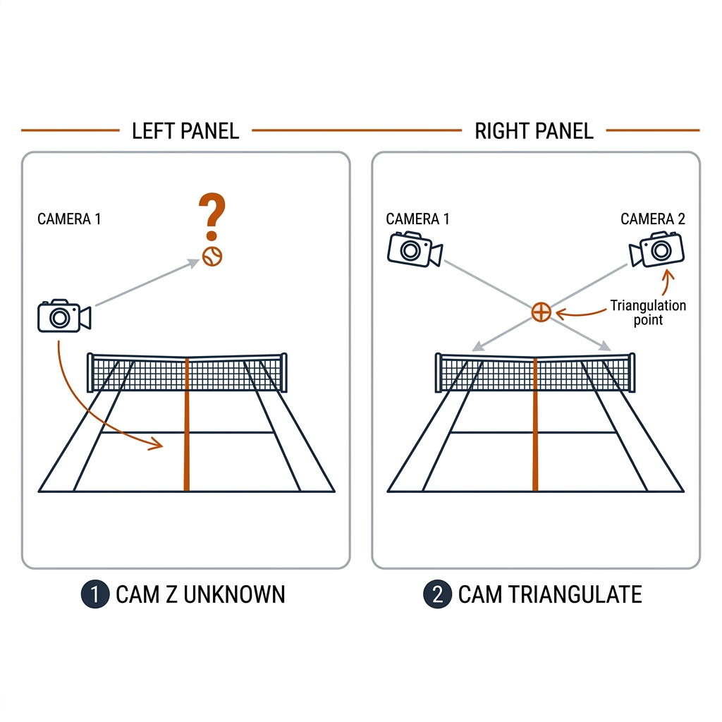
Multi-view is the honest fix: two calibrated views triangulate the ball outright, bounce points become geometry instead of inference, and true 3D speed replaces the fitted proxy. The costs are real — genlock or timestamp sync, per-camera calibration (C06/C07), doubled bandwidth and storage, and cross-view identity. The professional extreme solves the same problem by buying observations: Hawk-Eye-class systems run 340fps across 10–18 cameras and report ~2.6–3.6mm accuracy [secondary reporting; verify] — at that frame rate the exposure smear and inter-frame gap shrink until a simple tracker suffices. The book's stance: the physics prior is what you use when you cannot buy 340fps. For our fixtures the practical ladder is: pb-003-style fixed rigs → add one side camera for the kitchen plane (cheap, solves the bounce); nrl-001-style broadcast → single PTZ feed, no second view exists, so the carry model plus physics prior is the ceiling, and broadcast replay angles are the only triangulation you will ever get.
12.9 The Open Frontier
Spin and true speed are not recoverable from monocular video without sub-pixel geometry (the paddle-angle + spin-rate problem is partially open). Speed along the fitted path is recoverable with the physics prior; spin is not. Any product claiming spin from one camera is overclaiming.
The aliasing math makes "impossible" precise. Recreational-to-pro pickleball spin runs ~5–25 rev/s; the sampling theorem demands ≥2 samples per revolution, so 60fps footage aliases anything above 30 rev/s — and at 8–14px footprints with 1/60s smear there are no resolved surface features to sample anyway. The 40-hole pattern is visible only at ≥1/1000s shutter and ≥20px footprint. Spin from the book's current pb-003 footage is not a hard problem; it is excluded by the sampling theorem. The frontier sits in two places: event cameras, which track ball logos through microsecond-resolution polarity spirals (Nakabayashi et al., CVPRW 2024: up to 500 rev/s in table tennis; PATS 2025 localizes ball–racket impact at µs resolution) — both sensor-bound, not model-bound; and BlurBall (2026), which uses the motion blur itself as the signal [verify code availability]. The frame-camera fallback is inference from trajectory shape: §12.7's lift anomalies mean topspin dives harder than symmetric Magnus predicts, so a physics-fit inversion can estimate an effective $C_L$ per shot — a spin proxy with honest error bars, not a spin measurement.
For rugby the frontier statement is gentler: spiral rate and axis are observable at broadcast resolution when the ball is in flight (the ball is large), tumble vs spiral classification is a segmentation statistic, and the genuinely open problem is the contested ball — possession state through the ruck, which is a multi-person occlusion problem, not an aerodynamics one. In both sports, observing spin directly is a capture decision (shutter, footprint, frame rate, or a different sensor), never a model decision.
12.9b The 10 Use Cases: Applied Framework
Ten concrete jobs the ball-tracking stack performs, in three groups: shot quality and value (UC 01-04), physics calibration (UC 05-06), and adjudication and robustness (UC 07-10). Each case names the practical problem, the mechanism and the math, and pairs a pickleball and a rugby league application so the pipeline transfers. Evidence labels follow the book's discipline: measured (E-series), source-backed (paper), or [verify] (practitioner model).
Group A: Shot Quality & Value (UC 01-04)
UC 01 — Third-Shot Drop Apex & Net Clearance
The third-shot drop is the highest-leverage shot in pickleball — C22's ΔEPV boundary values it at +0.142 against the drive's -0.188 [verify — practitioner model] — and its quality is two numbers: did the arc peak on the hitter's side, and by how much did it clear the 0.86m net? The mechanism: take the physics-rectified trajectory of §12.6, fit the ballistic segment from contact to bounce, and read the apex $z^* = z_0 + v_z^2/2g$ plus the net clearance $c = z(x_{\text{net}}) - 0.86$ m. Both come from the fitted curve rather than any single noisy frame — the fit is the metrology. An attackable drop is one with $c > 15$ cm or an apex drifting to the kitchen side; an unattackable one peaks early and dies into the kitchen.
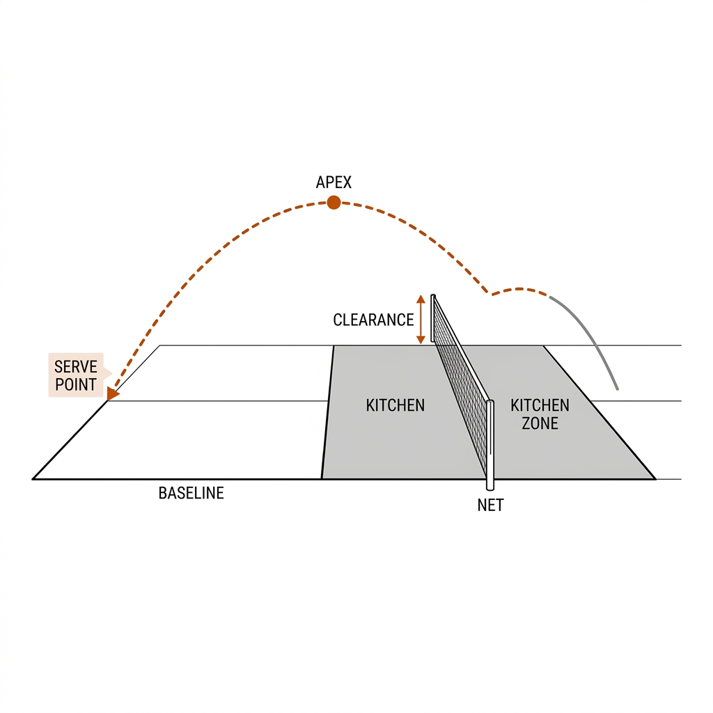
Payoff: coaching — apex side and clearance become the drill numbers for the most valuable shot in the sport, and the per-shot feed into C22's expected-point model.
UC 02 — The 40/20 Kick: Trajectory, Spin & the Bounce Cone
The 40/20 is rugby league's highest-skill territorial play: kicked from behind the team's own 40m line, the ball must bounce in-field and cross the touchline inside the opponent's 20m zone, earning the kicking team the scrum feed. It is a trajectory problem end to end: exit speed, launch angle, spiral stability, and — because the ball must bounce before going out — the bounce cone of §12.2b. The mechanism: classify spiral vs tumble from the ball mask's aspect-ratio oscillation (SAM 2, C09), then fit the matching drag regime — a spiral flies the $C_d \approx 0.18$ curve ($k \approx 0.008$ m⁻¹, six times lower than a pickleball's), a tumble flies $C_d \approx 0.55$ and wanders. The landing prediction is reported as a cone, and the call reduces to whether any in-cone path exits touch inside the 20m window.
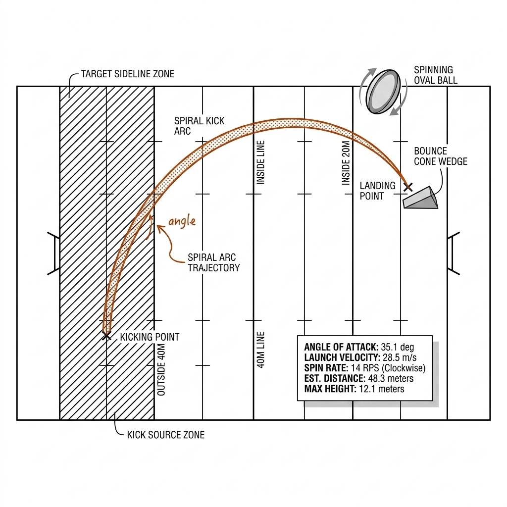
Payoff: tactical and officiating — kick-quality grading for recruitment, and a measurement-backed answer when the touch judge's angle is hopeless.
UC 03 — Speed-Gun Metrics: Serve km/h vs Punt km/h
Ball speed is the number every broadcast wants and the number monocular video most often gets wrong. The honest method: speed is the derivative of the fitted trajectory, $v = |\dot{\mathbf{x}}|$ in court coordinates, reported at named instants — at contact and at the bounce — with error bars from the fit, not the frame-to-frame pixel hop that the Z-limit (§12.8) inflates whenever the ball is airborne. On pb-003 that means serve-class figures around 112 km/h (31 m/s) at contact decaying to ~74 km/h by the bounce under $k \approx 0.045$ m⁻¹. The cross-check is a Pocket-Radar-class spot reading on ten drives [verify — hardware lab scheduled, §12.11]. For rugby the same machinery grades the kicking game: torpedo punt exit speed against hang time $t = 2v_z/g$ — the 4.5-5s bomb that lets the chase arrive is a tradeoff curve, not a single number.
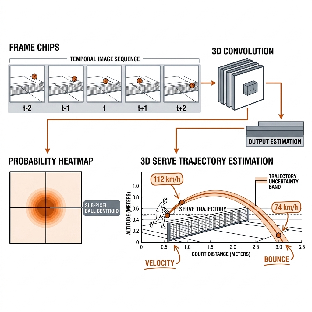
Payoff: broadcast and coaching — the C28 cockpit's live speed readout, earned honestly instead of inflated by the Z-limit.
UC 04 — Serve Spin: Proxy from Trajectory Shape
§12.9's verdict stands: spin from 60fps footage is excluded by the sampling theorem. But spin is not invisible — it is encoded in trajectory shape. Lindsey's anomalies (topspin lift systematically stronger than backspin at equal spin; backspin $C_L$ clustering near 0.2) mean a topspin serve dives measurably harder than symmetric Magnus predicts. The mechanism: per shot, fit $v_0$, launch angle, $C_d$, and an effective $C_L = C_L^{Magnus} + C_L^{gravity} + C_L^{internal}$ to the rectified trajectory; the residual lift term is the spin proxy. Publish it as "effective lift" with fit error bars — never as RPM. For rugby the analogue is observable directly: the ball is large, so spiral rate and axis wobble are measurable from the mask, and the tumble classification of UC 02 is itself the spin readout that matters for bounce prediction.
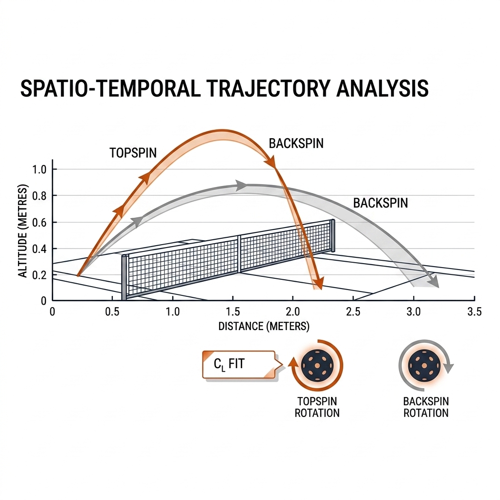
Payoff: coaching — a shot-level spin character per player without buying an event camera; the capture-spec route (C04) remains the answer when true RPM is required.
Group B: Physics Calibration (UC 05-06)
UC 05 — Drag Decay Measurement: Fitting Your Own C_d
Every downstream number — speed at bounce, apex, ΔEPV feed — inherits the drag coefficient, and §12.7's erratum showed what a wrong one does. So measure it instead of trusting a table. The mechanism: along a clean flight segment, sample fitted speeds $v_i$ at distances $x_i$; under $v(x) = v_0 e^{-kx}$ the regression $\ln v_i = \ln v_0 - k x_i$ is linear, and $C_d = 2mk/\rho A$ follows. That is Lindsey's RK4 method reduced to a least-squares line, and the acceptance check is the literature band: indoor $C_d \approx 0.45 \pm 0.09$, outdoor $0.33 \pm 0.08$ (86 free-flight trajectories, 300fps; self-published, corroborated by Steyn 2025). For rugby the same regression runs per attitude regime: gate spiral vs tumble first (UC 02), because pooling them fits a fiction — the two populations differ by 3×.
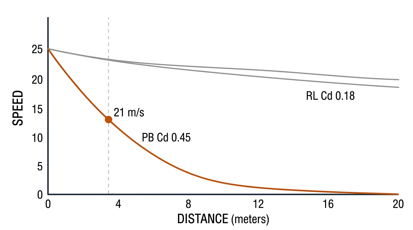
Payoff: infrastructure — the C24 simulator and every speed stat in the book inherit this coefficient; fitting it on your own footage is one afternoon of scipy.
UC 06 — Bounce Prediction: Point in Pickleball, Cone in Rugby
Predicting the bounce is the highest-value short-horizon forecast in both sports: it is where players move before the ball arrives. The mechanism is a bounce model appended to the ballistic integrator: at court-plane intersection, reflect with restitution $v_z^+ = -e\,v_z^-$ and horizontal retention $v_x^+ = \alpha v_x^- + \beta\omega$ — topspin kicks forward, backspin checks. The USA Pickleball ball spec (30-34 inches from a 78-inch drop) bounds $e \approx 0.62\text{–}0.66$ [verify — equipment spec]; the prediction is a point with a fitted uncertainty ellipse. Rugby inverts the honesty: a tumbling prolate spheroid has no bounce point, so the prediction is a cone whose half-angle is estimated from the tumble rate, and the honest output is a fielding zone, not a spot.
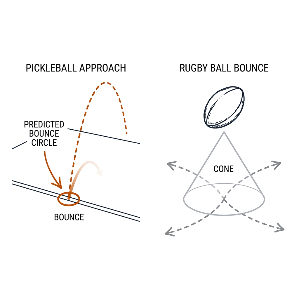
Payoff: tactical — anticipation metrics for C23's player models, and the bounce event rows that gate C19's event machine.
Group C: Adjudication & Robustness (UC 07-10)
UC 07 — Ball-Line Proximity: The Line Call as a Measurement
The kitchen-line call, the sideline, the baseline — every line call is a distance measurement with an uncertainty, and should be reported as one. The mechanism exploits §12.8's inversion: at the bounce frame the homography is exactly right, so project the bounce point, compute the signed distance to the line $d = |ax + by + c|/\sqrt{a^2+b^2}$, and propagate the uncertainty — centroid RMSE (1.42px, E10) through the calibration Jacobian gives $\sigma_d$ in centimeters. The adjudication rule: call IN or OUT only when $|d| > 3\sigma_d$; inside that band the honest output is "too close to call," which is what the 68%/84% Bath-grade humility (§12.8) looks like applied to geometry. Rugby's versions are the touchline on kicks (UC 02's 40/20 exit) and the try-line grounding.
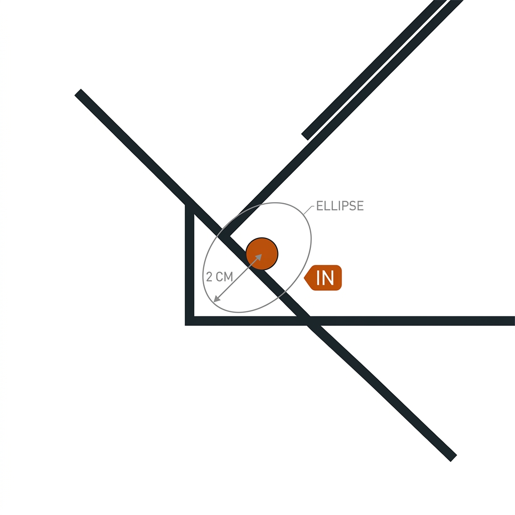
Payoff: officiating — a defensible call with a printed error bar replaces the argument; feeds C03's rules layer.
UC 08 — Ball-in-Ruck Occlusion: The Carry State Machine
Rugby's defining ball problem is a 40-80 frame hole in which the ball is not ballistic but buried. No physics prior spans that; the mechanism is a state machine alongside the track: carried (ball bound to the carrier's torso region), contested (bound to the ruck centroid while bodies pile over it), in flight (ballistic prior active), with hand-off events at the play-the-ball, the dummy-half pickup, and every pass or kick. The play-the-ball clock — the ruck-speed number rugby analytics runs on — falls out of the state transitions for free: tackle-state entry to dummy-half release. Pickleball's version is the same machinery at 2-10 frame scale: the body block at the kitchen line and the contact merge, both bridged by the §12.6b ellipse contract instead of a state machine.
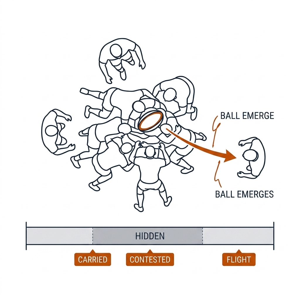
Payoff: tactical — ruck speed and PTB bands feed C19's event rows and C28's DLSM metrics; possession state makes rugby's ball track continuous for the first time.
UC 09 — Multi-Camera Ball Fusion
§12.8b's ladder ends here: two calibrated views turn the ball from a bearing into a point. The mechanism: detect heatmap peaks independently per view, match candidates by epipolar constraint — a true ball detection in view A must lie on the epipolar line of its view-B partner, so E10's residual false positives (net flutter, paddle tips) die unmatched — then triangulate $X^* = \arg\min_X \sum_i \|\pi_i(X) - x_i\|^2$. Three purchases follow at once: true 3D position (the Z-limit dissolves), bounce points as geometry instead of inference (UC 06/07 upgrade from fitted to measured), and true 3D speed replacing the UC 03 proxy. The budget version for pickleball: one added side camera covering the kitchen plane solves the calls that matter. For broadcast rugby there is no second view; replay angles are the only fusion you will get.
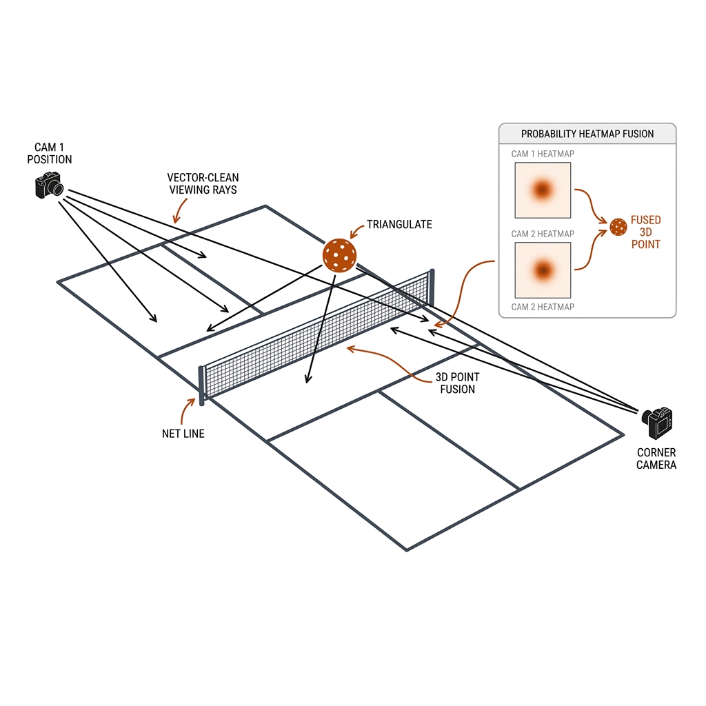
Payoff: officiating and infrastructure — the upgrade path from inference to geometry; this is C14's multi-view chapter applied specifically to the ball.
UC 10 — Tracker Drift Correction with Bounce Anchors
Every filter drifts: integration error, calibration wobble (C07), and the unidentifiable drag interaction of §12.6 accumulate until the fitted trajectory silently departs from the true one. The correction uses the chapter's own event layer: bounces and contacts are innovation spikes where the physics resets — at a bounce the ball is at z = 0 with a reflected velocity, a hard state constraint no integration error survives. The mechanism: run the constant-acceleration filter forward, but at each detected anchor re-initialize the state (position pinned to the homography-valid bounce point, velocity re-seeded by the restitution model of UC 06), and smooth the whole segment with an RTS backward pass so corrections propagate both ways. Uncertainty grows between anchors and collapses at them — the sawtooth error profile is the signature of a healthy track.
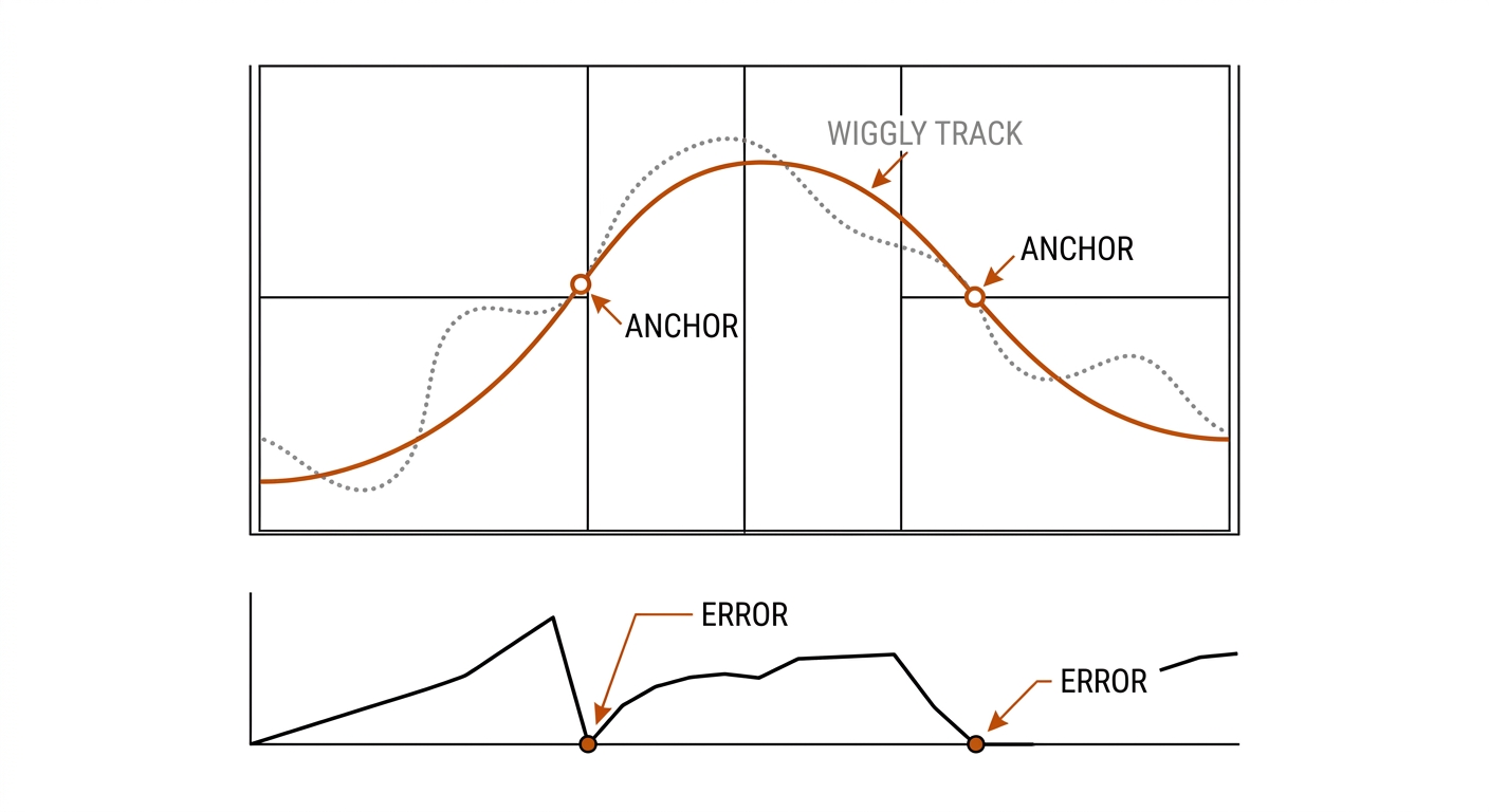
Payoff: infrastructure — every downstream statistic inherits the track's drift unless something resets it; the bounce anchors are that something, and they are free.
12.9c The Ecosystem & Runnable Skeleton
The libraries a practitioner actually reaches for around the TrackNet core, with the sport-specific job of each:
| Tool | License | Role | Pickleball use | Rugby league use |
|---|---|---|---|---|
| TrackNetV2 (2020) | ⚠️ no license file [verify] | Fine-tune backbone | 500-frame fine-tune base (§12.11) | n/a — scale is not the wall |
| TrackNetV3 (2023) | NOASSERTION [verify] | Occlusion rectification | Contact-merge window repair | Kick-flight gap repair |
| TrackNetV4 (ICASSP 2025) | Paper only, no code [verify] | Motion-attention plugin | The E10 → learned upgrade path | Motion maps after GMC (C07) |
| TrackNetV5 (Dec 2025) | Proprietary SDK/weights | Architecture reference | Signed motion fields — reimplement | Same idea; never the weights |
| WASB-SBDT (BMVC 2023) | MIT | Protocol + constant-accel tracker | First public pickleball benchmark row | Transfers structurally from soccer |
| MonoTrack (2022) | No release [verify] | Monocular 3D template | Net-plane Z-checkpoint fit (§12.8b) | n/a — broadcast single view |
| RacketVision (2025) | MIT | Ball + paddle schema | 6-point paddle pose annotation | — |
| SAM 2 (2024) | Apache-2.0 | Equipment & ball masks | Paddle-face angle at contact | Spiral/tumble aspect-ratio signal |
The starting skeleton — E10's temporal filter plus the ballistic fit — is deliberately boring; the full lab version with sub-pixel readout and the drag scan lives in lab/w3_lab_ball.py:
import cv2, numpy as np
from scipy.optimize import least_squares

def temporal_energy(f0, f1, f2, area=(6, 150), min_circ=0.4):
    """E10: AND of consecutive absdiffs -> candidate ball centers."""
    d = cv2.bitwise_and(cv2.absdiff(f1, f0), cv2.absdiff(f2, f1))
    m = cv2.threshold(cv2.cvtColor(d, cv2.COLOR_BGR2GRAY), 25, 255, 0)[1]
    for c in cv2.findContours(m, cv2.RETR_EXTERNAL, cv2.CHAIN_APPROX_SIMPLE)[0]:
        a, p = cv2.contourArea(c), cv2.arcLength(c, True)
        if area[0] <= a <= area[1] and p > 0 and 4*np.pi*a/p**2 > min_circ:
            M = cv2.moments(c)
            yield M['m10']/M['m00'], M['m01']/M['m00']

G, K = 9.81, 0.045   # gravity; drag k = 0.5*Cd*rho*A/m, 26g 74mm ball
def residual(p, pts, t):
    x0, y0, vx0, vy0 = p          # court meters, z=0 plane segment
    dt = t - t[0]
    x = x0 + vx0*(1 - np.exp(-K*dt))/K          # drag along flight
    y = y0 + vy0*dt - 0.5*G*dt**2               # gravity vertical
    return (np.stack([x, y], 1) - pts).ravel()

def fit_segment(px_pts, t, H):
    """Project to meters via homography H, then fit v0/angle; scan K for Cd."""
    pts = (H @ np.c_[px_pts, np.ones(len(px_pts))].T).T
    pts = pts[:, :2] / pts[:, 2:]
    v0 = np.diff(pts[:5], axis=0).mean(0) / (t[1] - t[0])
    return least_squares(residual, [pts[0,0], pts[0,1], *v0], args=(pts, t))
12.9d What This Adds to the Pipeline
The ten use cases are the ball layer applied across the book's five verbs, and each one lands in an existing chapter rather than standing alone: UC 01's apex and clearance feed C22's ΔEPV shot valuation; UC 03's speed readouts and UC 08's ruck clock feed the C28 cockpit's live bands; UC 05's fitted $C_d$ parameterizes the C24 simulator; UC 06 and UC 07 emit the bounce and line-call events that gate C19's event rows and C03's rules layer; UC 09 is C14's multi-view machinery applied to the one object that needs it most; UC 04's honest spin proxy defers to C04's capture spec when true RPM is required; and UC 10 keeps every one of those consumers honest by pinning the track they all inherit. The labels stay where the evidence is: E04/E10 measured, Lindsey/Seo/Alam source-backed, and [verify] wherever a practitioner model has not yet earned a number.
12.10 The Ball-Tracking Recipe (Copy This)
- Capture right: ≥1/1000s shutter (C04 math: 5px blur at 1/1000), 30fps minimum, 60fps for ball work — remember the 25Hz hop is ~200px at drive speed (§12.4b).
- Label a fixture: 500 frames with ball centers, split by rally not by frame (the G0.5 dataset contribution — labels CC-BY-4.0).
- Baseline first: the 3-frame temporal energy filter (E10: 0.814 precision@50px, 76.2% continuity) — 30 lines of OpenCV, no training. On broadcast rugby, run global motion compensation (C07) first or the baseline sees only camera pan.
- Then the deep model: TrackNetV4 fine-tune on the 500 frames (Colab T4; license [verify]; the V5 successor has proprietary weights — reimplement the signed-motion-fields idea, never depend on the SDK).
- Physics-rectify: Kalman or least-squares fit with gravity + drag (the 3.7× MSE gain measured) — gap bridging, 3σ outlier veto, innovation spikes as bounce/contact candidates.
- Branch by sport: pickleball — flight tracking with the ballistic prior, bounce detector gating PBN rows. Rugby league — ball-carry state machine (carried / contested / in flight), spiral-tumble classification from mask aspect ratio, bounce cones not bounce points.
- For bounce/contact adjudication: escalate to multi-view (chapter 14) — the Z limit means a single camera reports a trajectory, not a bounce point.
- Honesty gate: fit the trajectory, not the launch physics. (Our fit recovered 24.8 m/s for a true 20.0 — the drag interaction is unidentifiable at this noise.) Report precision with its pixel tolerance, continuity with its clip, and any spin number with the capture spec that made it observable.
12.11 What I Would Measure Next
- E10 rerun + cross-sport extension (M4, pure OpenCV): reproduce the E10 table on pb-003, then run the same filter on (a) nrl-001 kick sequences — testing the C08 prediction that rugby's ball problem is occlusion, not scale — and (b) a dink-heavy pickleball clip for the slow-apex failure mode. Emit a per-class false-positive table (net flutter / paddle tips / shadows) to size the physics-gate veto.
- Ballistic-fit inversion (M4, scipy RK4 + least_squares): fit $v_0$, launch angle, $C_d$, effective $C_L$ per rally segment between detected bounces; the fitted $C_d$ distribution should land near Lindsey's 0.33–0.45 band; radar spot-check 10 drives if hardware is available.
- Bounce detector v1: innovation-spike + homography-consistency detector against 30 hand-labeled bounces on pb-003; ≥90% precision before it gates any PBN event rows.
- Label 500 frames with ball centers (the G0.5 dataset work; E10 pre-annotates, humans correct), fine-tune TrackNetV4 on Colab. Acceptance bar: beat E10's 0.814 precision@50px on held-out rallies; the projection target is 0.938 / 91.5% continuity. Report the same-match vs cross-match generalization gap honestly (TrackNet 2019 lost 14 F1 points there).
- WASB-SBDT baseline on the same labels — the first public pickleball row on the cross-sport protocol.
- RacketVision-schema pilot: 100 frames of ball + 6-point paddle pose + contact events, with annotation cost measured in minutes/frame to size the real dataset effort.
- Monocular Z-fit test: the net-plane checkpoint fit of §12.8b on pb-003 rallies — first pickleball numbers for the MonoTrack-style constraint.
12.12 Sources
- TrackNet (Huang et al. 2019, arXiv:1907.03698); TrackNetV2 (NYCU technical report 2020); TrackNetV3 (MMAsia 2023, github.com/qaz812345/TrackNetV3, license NOASSERTION [verify]); TrackNetV4 (ICASSP 2025, arXiv:2409.14543; no official code [verify]); TrackNetV5 (arXiv 2512.02789, proprietary SDK/weights); WASB-SBDT (BMVC 2023, arXiv:2311.05237, MIT).
- MonoTrack (monocular 3D shuttlecock, arXiv:2204.01899); RacketVision (Nov 2025, arXiv:2511.17045, MIT) — ball + racket pose schema.
- Aerodynamics: Lindsey (Tennis Warehouse, May 2025, self-published, corroborated by Steyn 2025 and Rossmann & Rau 2007); Seo et al. (ASME J. Appl. Mech. 79(2)) and Alam et al. (RMIT) for rugby ball drag vs yaw.
- Frontier: Nakabayashi et al. (CVPRW 2024, event-based spin to 500 rev/s); PATS (arXiv:2506.08327, µs impact localization); BlurBall (arXiv 2604.24033 [verify code]); Bath 2025 head-on-head framework (Injury Prevention, PMID 39832883; 68%/84% [verify league vs union]).
- Book-internal: E04 (experiments/e04-ball), E10 (experiments/e10-ball-temporal), C12 lab (
lab/w3_lab_ball.py); C03 (rules), C04 (blur = v·t, 1/1000s rule), C06 (Z-limit), C07 (moving-camera calibration), C08 (class distribution), C09 (SAM boundary), C14 (multi-view).